260607 Data Structures Dana Shapira Hash Tables Element

26/06/07 Data Structures Dana Shapira Hash Tables

Element Uniqueness Problem n Let n Determine whethere exist i j such that xi=xj n Sort Algorithm n Bucket Sort for (i=0; i<m; i++) O(m) T[i]=NULL; O(n) for (i=0; i<n; i++){ if (T[xi]= = NULL) T[xi]= i else{ output (i, T[xi]) return; } } O(m+n) : סיבוכיות What happens when n is large or when we are dealing with real numbers? ?

Hash Tables h טבלאות גיבוב n Notations: n U universe of keys of size |U|, n K an actual set of keys of size n, n T a hash table of size O(m) U n Use a hash-function h: U {0, …, m-1}, h(x)=i that computes the slot i in array T where element x is to be stored, for all x in U. n h(k) is computed in O(|k|) = O(1). Set of array indices מספר המפתחות n גדול הטבלה m מניחים שזמן החישוב הוא קבוע h(x 1) h(x 2) h(x 3) h(x 4) x 1 x 2 x 3 x 4
=x mod 10 (what is")
Example 0 n h: U {0, …, m-1} m=10 h(x)=x mod 10 (what is m? ) פונקצית הגיבוב היא על input: 17, 62, 19, 81, 53 : נקבל בעיית התנגשות 82 אם נרצה להכניס את n n n Collision: x ≠ y but h(x) = h(y). 82!=62 but h(82)=h(62)=2 m « |U|. קטן ממש ביחס לגודל היקום m Solutions: 1. Chaining 2. Open addressing 1 81 2 62 3 4 53 5 6 7 8 17 9 19

Collision-Resolution by Chaining שרשור באמצעות רשימה מקושרת חד כיוונית 1 81 62 12 53 17 37 57 19 n n n Insert(T, x): Delete(T, x): Search(T, x): Insert new element x at the head of list T[h(x. key)]. Delete element x from list T[h(x. key)]. <- פעולה של הורדת איבר מרשימה חד כיוונית Search list T[h(x. key)].
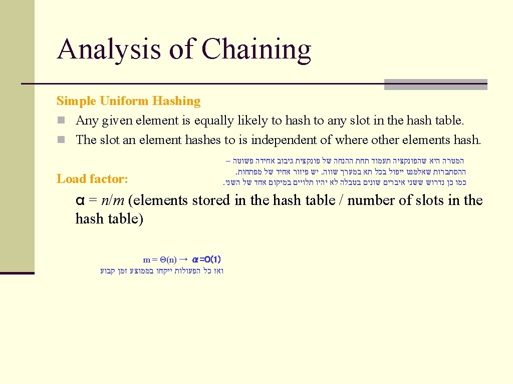

Analysis of Chaining שרשור - ניתוח סיבוכיות : בשני המקרים – חיפוש מוצלח וחיפוש כושל – נקבל סיבוכיות של משמש לחישוב פונ' הגיבוב עצמה 1 – כאשר ה , Θ(1+α) n Theorem: In a hash table with chaining, under the assumption of simple uniform n n hashing, both successful and unsuccessful searches take expected time Θ(1+α) on the average, where α is the hash table load factor. Proof: Unsuccessful Search: Under the assumption of simple uniform hashing, any key k is equally likely to hash to any slot in the hash table. The expected time to search unsuccessfully for a key k is the expected time to search to the end of list T[h(k)] which has expected length α. expected time - O(1 + α) including time for computing h(k). Successful search: The number of elements examined during a successful search is 1 more than the number of elements that appear before k in T[h(k)]. מעבר למקום V הבא ברשימה איברים i-1 עוברים על . i – ומוצאים באיבר ה נעשית כי מדובר n – החלוקה ב בממוצע expected time - O(1 + α) Θ(1+α) ומקבלים α /2> וגם α/4< המספר הזה ^ מקיים : סיבוכיות n Corollary: If m = O(n), then Insert, Delete, and Search take expected constant time.
 = x mod m m = 2 k")
The Division Method Hash function: h(x) = x mod m m = 2 k h(x) = the lowest k bits of x. לא לוקחים את כל הספרות – מתרחק מהנחת הגיבוב האחיד על הטבלה n. Heuristic: : אלא , כנ"ל m לכן לא נבחר m = prime number not too close to a power of 2 n
 = m (cx mod 1) , for some")
The Multiplication Method Hash function: h(x) = m (cx mod 1) , for some 0 < c < 1 ^ מה שמופיע אחרי הנקודה בשבר n Optimal choice of c depends on input distribution. c מקודם הפונקציה היתה תלויה בגודל הטבלה וכעת תלויה בקבוע , הפונק' הזו יותר טובה n. Heuristic: Knuth suggests the inverse of the golden ratio as a value that works well: . כזה יאפשר גיבוב אחיד על פני הטבלה c , עפ"י קנוט Example: מפתח גודל טבלה x=123, 456, m=10, 000 h(x) = 10, 000 ·(123, 456· 0. 61803… mod 1) = = 10, 000 ·(76, 300. 0041151… mod 1) = = 10, 000 · 0. 0041151… = 41. 151. . . = 41
 = m (cx mod 1) . ניתן")
Efficient Implementation of the Multiplication Method h(x) = m (cx mod 1) . ניתן לבצע זאת עם פעולות של ביטים , c ע"י בחירה מתאימה של קבוע . הביטים העליונים במילה התחתונה p נסתכל על , בסופו של דבר w bits n. Let w be the size of a machine word n. Assume that key x fits into a machine word n. Assume that m = 2 p * n. Restrict ourselves to values of c of the form c = s / 2 w n. Then cx = sx / 2 w : ניקח nsx is a number that fits into two machine words מילות מכונה 2 - נכנס לכל היותר ב Sx nh(x) = p most significant bits of the lower word w bits Fractional part Integer part after multiplying by m = 2 p w bits p bits
 = m (cx mod 1) מפתח nx = 123456, p = 14,")
Example h(x) = m (cx mod 1) מפתח nx = 123456, p = 14, m = 214 32 bit = 16384, w = 32, n. Then sx = (76300 ⋅ 232) + 17612864 n. The 14 most significant bits of 17612864 are 67; that is, h(x) = 67 x = 0000 0001 1110 0010 0100 0000 s = 1001 1110 0011 0111 1001 1011 1001 sx = 0000 0001 0010 1010 0000 1100 : 123456 הרצף הבינארי של : 2654435769 הייצוג של 0000 0001 0000 1100 0000 0100 0000 h(x) = 00 0000 0100 0011 = 67 ( כי לא למדנו ייצוג בינארי של מספרים , )די דילגנו

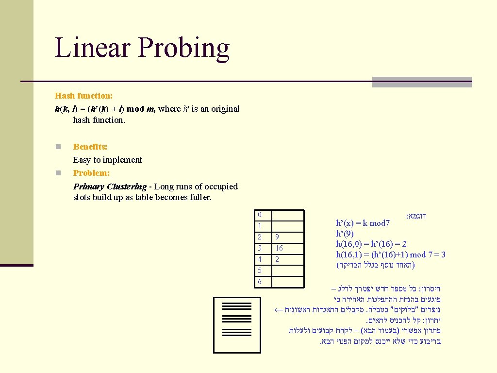
Open Addressing n. All elements are stored directly in the hash table. ➥Load factor α cannot exceed 1. n. If slot T[h(x)] is already occupied for a key x, we probe alternative locations until we find an empty slot. n. Searching probes slots starting at T[h(x)] until x is found or we are sure that x is not in T. n. Instead of computing h(x), we compute h(x, i) →. זהו הנידסיון להכניס איבר i=0 בפעם הראשונה n i -the probe number. אחרת אם. צריך דגל שיסמן – תפוס לצרכי חיפוש אך פנו לצרכי הכנסה. המחיקה לא מתבצעת באופן ישיר לא יהיה לנו איך להגיע לאיבר , I – ואז מחקנו את האיבר מ , II – ואיבר שני ב I – למשל הכנסנו איבר ראשון ב . II – ב I h(x) II
 = (h'(k) + c 1 i + c")
Quadratic Probing Hash function: h(k, i) = (h'(k) + c 1 i + c 2 i 2) mod m, where h' is an original hash function. n Benefits: No more primary clustering n Problem: Secondary Clustering - Two elements x and y with h'(x) = h'(y) have same probe sequence. נוצרת התאגדות שניונית

Double Hashing פתרון נוסף – שתי פונקציות גיבוב hash ' חסרון – צורך בשתי פונ Hash function: = מס' הדגימה i h(k, i) = (h 1(k) + ih 2(k)) mod m, where h 1 and h 2 are two original hash functions. n h 2(k) has to be prime w. r. t. m; that is, gcd(h 2(k), m) = 1. n Two methods: Choose m to be a power of 2 and guarantee that h 2(k) is always odd. h 2(k)!=0 Choose m to be a prime number and guarantee that h 2(k) < m. n Benefits: אחרת לא נגיע לכל המקומות בטבלה No more clustering n Drawback: More complicated than linear and quadratic probing
, …, h(k,")
Analysis of Open Addressing n Uniform hashing: The probe sequence h(k, 0), …, h(k, m – 1) is equally likely to be any permutation of 0, …, m – 1. הנחה חדשה במקום הנחת הגיבוב הפשוט – הסתברות קבל כל אחד מהמספרים תהיה אחידה n Theorem: In an open-address hash table with load factor α < 1, the expected number of probes in an unsuccessful search is at most 1 / (1 – α), assuming uniform hashing. Proof: Let X be the number of probes in an unsuccessful search. Ai = “there is an i-th probe, and it accesses a non-empty slot” ( )הוכחה בהסתברות – עברנו על זה באופן כללי
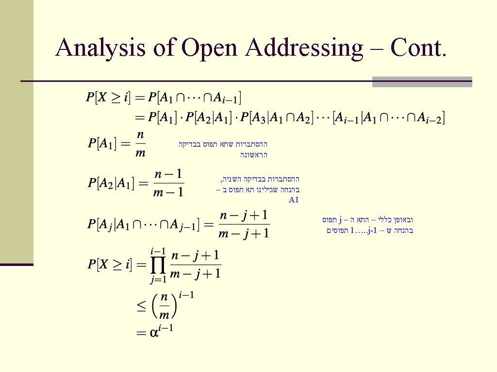

Analysis of Open Addressing – Cont. Corollary: The expected number of probes performed during an insertion into an open-address hash table with uniform hashing is 1 / (1 – α).

Analysis of Open Addressing – Cont. Theorem: Given an open-address hash table with load factor α < 1, the expected number of probes in a successful search is (1/α) ln (1 / (1 – α)), assuming uniform hashing and assuming that each key in the table is equally likely to be searched for. n A successful search for an element x follows the same probe sequence as the insertion of element x. n Consider the (i + 1)-st element x that was inserted. n The expected number of probes performed when inserting x is at most n Averaging over all n elements, the expected number of probes in a successful search is

Analysis of Open Addressing – Cont.

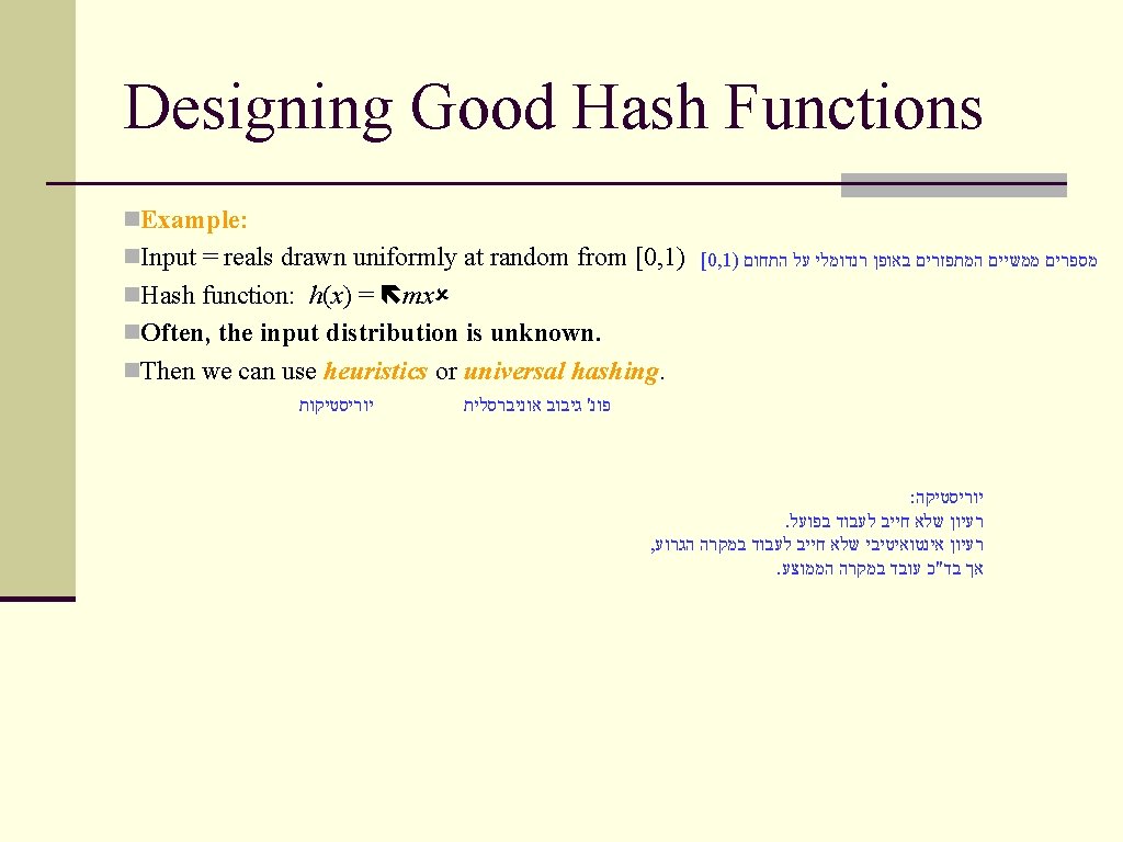
Universal Hashing . גיבוב אוניברסלי משפחות של פונקציות גיבוב – בוחרים באופן רנדומלי פונ' גיבוב . ומבצעים את כל הפעולות איתה n. A family of hash functions is universal if for each pair k, l of keys, there at most | | / m functions in such that h(k) = h(l). n. This means: For any two keys k and l and any function h chosen uniformly at random, the probability that h(k) = h(l) is at most 1/m ההסתברות להתנגשות היא , לכל זוג מפתחות n P= (| | / m )/ | | =1/m n. This is the same as if we chose h(k) and h(l) uniformly at random from [0, m – 1]. לא עברנו על הוכחות הסיבוכיות בהמשך

Analysis of Universal Hashing Theorem: For a hash function h chosen uniformly at random from a universal family , the expected length of the list T[h(x)] is α if x is not in the hash table and 1 + α if x is in the hash table. Proof: Indicator variables: Yx = the number of keys ≠ x that hash to the same slot as x

Analysis of Universal Hashing Cont. If x is not in T, then |{y T : x ≠ y}| = n. Hence, E[Yx] = n / m = α. If x is in T, then |{y T : x ≠ y} = n – 1. Hence, E[Yx] = (n – 1) / m < α. The length of list T[h(x)] is one more, that is, 1 + α.
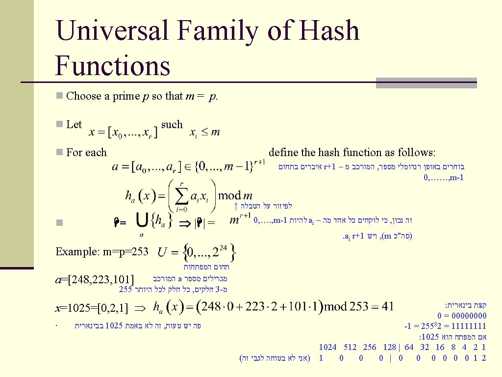

Universal Family of Hash Functions Theorem: The class is universal. Proof: Let such that x ≠ y, w. l. o. g n For all a 1, …, ar there exists a single a 0 such that n For all n there exists a single w such that z·w=1(mod m) for mr values , הוא שדה Zp – למדנו ש יש הופכי 0 - ולכן לכל מס' שונה מ n The number of hash functions h in , for which h(k 1) = h(k 2) is at most mr/ mr+1 =1/m

Universal Family of Hash Functions Choose a prime p so that m < p. For any 1 ≤ a < p and 0 ≤ b < p, we define a function ha, b(x) = ((ax + b) mod p) mod m. Let Hp, m be the family Hp, m = {ha, b : 1 ≤ a < p and 0 ≤ b < p}. Theorem: The class Hp, m is universal. ולכן תפוס לצרכי חיפוש , 133 מחקנו את : דוגמא h(k, i) = (h 1(k) + ih 2(k))mod 11 h 1(k) = k mod 11 h 2(k) = k md 5 + 1 אחרת , )האחד כדי שפונ' הגיבוב השניה תהיה שונה מאפס i )לא יקודם 0 39 1 133 2 3 4 37 5 6 89 7 67 8 9 10 97 insert(133) 97 89 תפוס – משתמשים בפונ' השנייה 39 תפוס – משתמשים בפונ' השנייה h(37, 0) = 4 h(67, 0) = 1 ! תפוס h(67, 1) = 4 ! תפוס h(67, 2) = 1+2 x 3 = 7 deleted(133) search(189) h(89, 0) = 1 h(89, 1)

Summary n Hash tables are the most efficient dictionaries if only operations Insert, Delete, and n n n Search have to be supported. If uniform hashing is used, the expected time of each of these operations is constant. Universal hashing is somewhat complicated, but performs well even for adversarial input distributions. If the input distribution is known, heuristics perform well and are much simpler than universal hashing. For collision-resolution, chaining is the simplest method, but it requires more space than open addressing. Open addressing is either more complicated or suffers from clustering effects.
- Slides: 28