258 Optimality Principle Assume that optimal path is

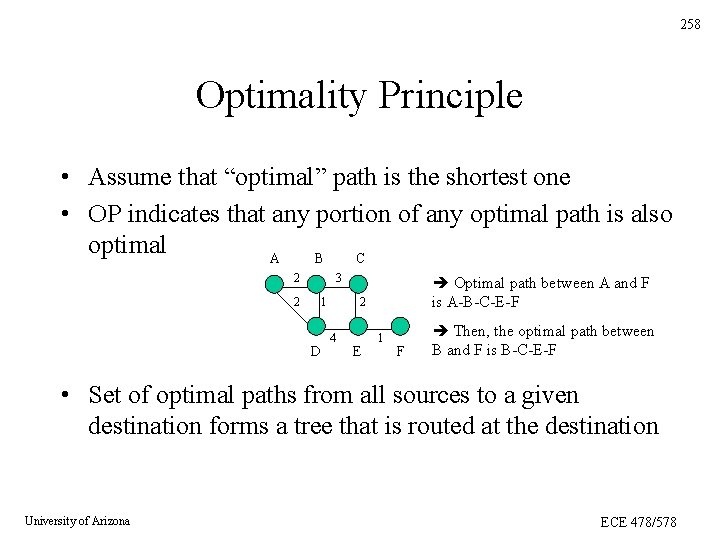
258 Optimality Principle • Assume that “optimal” path is the shortest one • OP indicates that any portion of any optimal path is also optimal A B C 2 2 3 1 D Optimal path between A and F is A-B-C-E-F 2 4 E 1 F Then, the optimal path between B and F is B-C-E-F • Set of optimal paths from all sources to a given destination forms a tree that is routed at the destination University of Arizona ECE 478/578

259 Shortest Path Algorithm • “Shortest” in the sense of distance (e. g. , total delay) • Assume that distance is “additive” • Two approaches to computing the shortest path: – Dijkstra’s algorithm (basis for link-state routing) – Bellman-Ford algorithm (basis for distance-vector routing) University of Arizona ECE 478/578

260 Dijkstra’s Algorithm • Goal: find the shortest path from a given source to all destinations • Network is represented by a graph G(V, E), where – V: set of nodes – E: set of links (edges) • Assume that each link is associated with a delay value • Starting from the source node, the algorithm “discovers” remaining node in the order of their distances from the source University of Arizona ECE 478/578

261 Dijkstra’s Algorithm (Cont. ) • Each node v V is associated with a label: – Current best distance from source s to v – Previous node from which distance was obtained • Initially, all labels are tentative • If the distance is not known yet, it is set to infinity • In each iteration, the algorithm chooses a working node from set of nodes with tentative nodes – Working node is one with smallest distance among tentatively labeled nodes – Its label now becomes permanent University of Arizona ECE 478/578

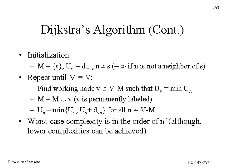
262 Dijkstra’s Algorithm (Cont. ) • Variables: – V: set of nodes in the graph – s: source node – dij: link cost from node i to node j (= if i is not a neighbor of j) – M: set of permanently labeled nodes – Un: current distance from s to node n University of Arizona ECE 478/578

263 Dijkstra’s Algorithm (Cont. ) • Initialization: – M = {s}, Un = dsn , n s (= if n is not a neighbor of s) • Repeat until M = V: – Find working node v V-M such that Uv = min Un – M = M v (v is permanently labeled) – Un = min{Un, Uv+ dvn} for all n V-M • Worst-case complexity is in the order of n 2 (although, lower complexities can be achieved) University of Arizona ECE 478/578

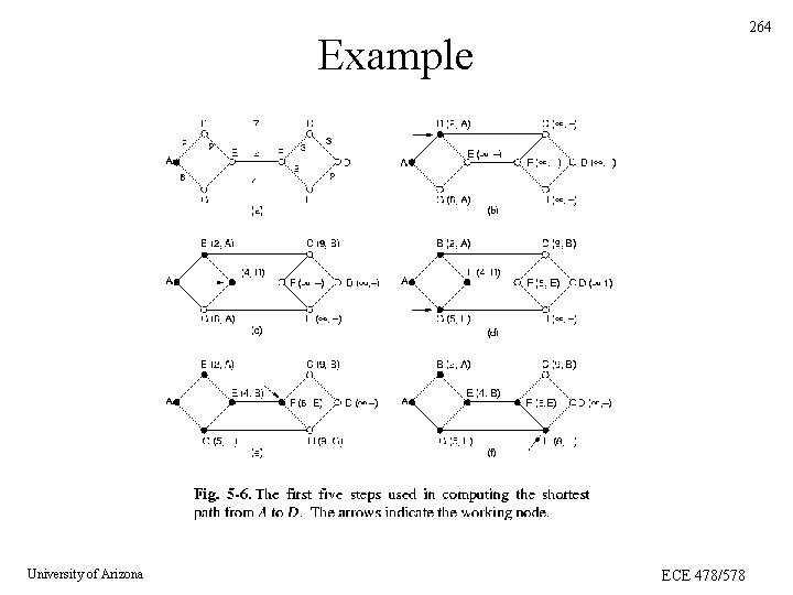
264 Example University of Arizona ECE 478/578

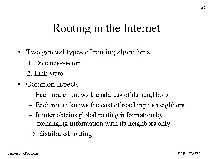
265 Routing in the Internet • Two general types of routing algorithms 1. Distance-vector 2. Link-state • Common aspects – Each router knows the address of its neighbors – Each router knows the cost of reaching its neighbors – Router obtains global routing information by exchanging information with its neighbors only distributed routing University of Arizona ECE 478/578

266 Routing in the Internet (Cont. ) • Fundamental difference – Distance-vector: a node informs its neighbors of its “distance” to every other node in the network – Link-state: a node tells every other node in the network of its “distance” to its neighbors – Distance can be interpreted in different ways University of Arizona ECE 478/578

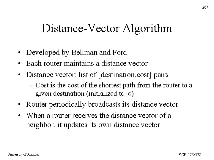
267 Distance-Vector Algorithm • Developed by Bellman and Ford • Each router maintains a distance vector • Distance vector: list of [destination, cost] pairs – Cost is the cost of the shortest path from the router to a given destination (initialized to ) • Router periodically broadcasts its distance vector • When a router receives the distance vector of a neighbor, it updates its own distance vector University of Arizona ECE 478/578

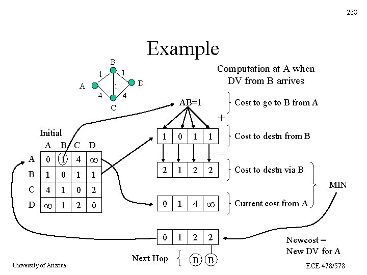
268 Example B A Computation at A when DV from B arrives 1 1 D 1 4 4 AB=1 C Initial A B C D A 0 1 4 B 1 0 1 1 C 4 1 0 2 D 1 2 0 University of Arizona Cost to go to B from A + 1 0 1 Cost to destn from B 1 = 2 1 2 2 Cost to destn via B MIN 0 1 4 0 1 2 2 B B Next Hop Current cost from A Newcost = New DV for A ECE 478/578

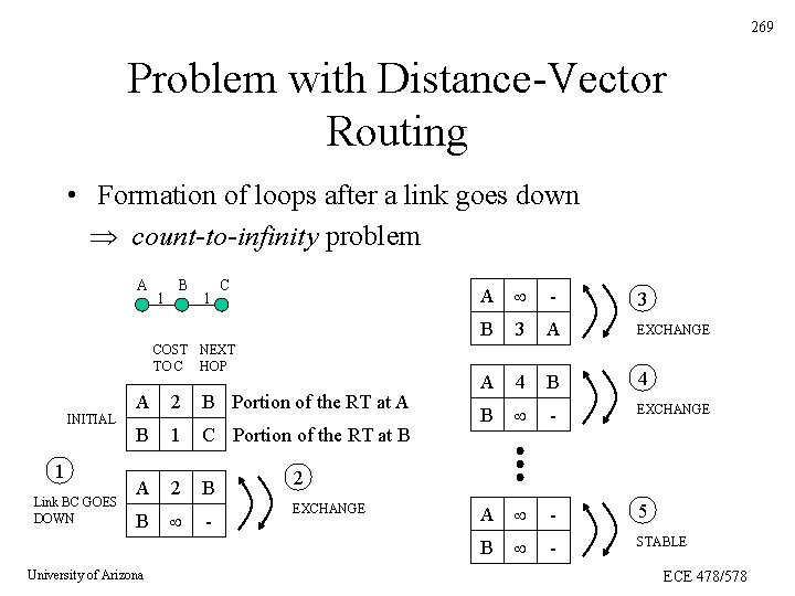
269 Problem with Distance-Vector Routing • Formation of loops after a link goes down count-to-infinity problem A 1 B 1 C COST NEXT TO C HOP INITIAL 1 Link BC GOES DOWN A 2 B Portion of the RT at A B 1 C Portion of the RT at B A 2 B B - University of Arizona A - 3 B 3 A EXCHANGE A 4 B - EXCHANGE A - 5 B - STABLE 2 EXCHANGE ECE 478/578

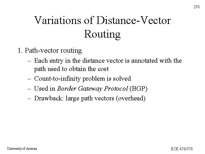
270 Variations of Distance-Vector Routing 1. Path-vector routing – Each entry in the distance vector is annotated with the path used to obtain the cost – Count-to-infinity problem is solved – Used in Border Gateway Protocol (BGP) – Drawback: large path vectors (overhead) University of Arizona ECE 478/578

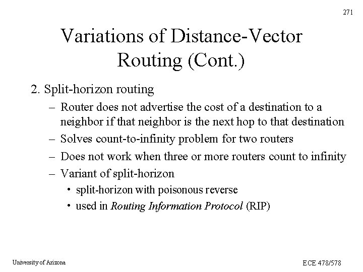
271 Variations of Distance-Vector Routing (Cont. ) 2. Split-horizon routing – Router does not advertise the cost of a destination to a neighbor if that neighbor is the next hop to that destination – Solves count-to-infinity problem for two routers – Does not work when three or more routers count to infinity – Variant of split-horizon • split-horizon with poisonous reverse • used in Routing Information Protocol (RIP) University of Arizona ECE 478/578

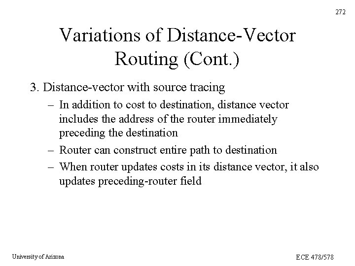
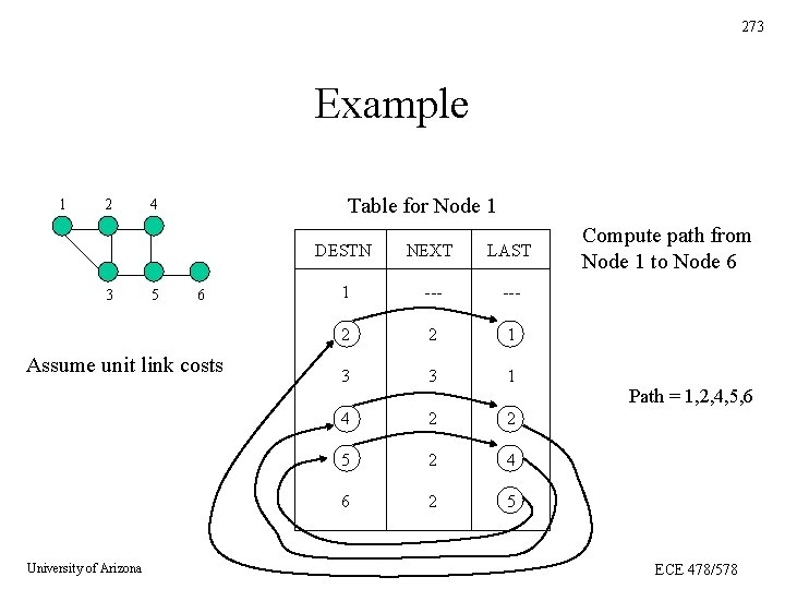
272 Variations of Distance-Vector Routing (Cont. ) 3. Distance-vector with source tracing – In addition to cost to destination, distance vector includes the address of the router immediately preceding the destination – Router can construct entire path to destination – When router updates costs in its distance vector, it also updates preceding-router field University of Arizona ECE 478/578

273 Example 1 2 3 Table for Node 1 4 5 6 Assume unit link costs University of Arizona DESTN NEXT LAST 1 --- 2 2 1 3 3 1 4 2 2 5 2 4 6 2 5 Compute path from Node 1 to Node 6 Path = 1, 2, 4, 5, 6 ECE 478/578

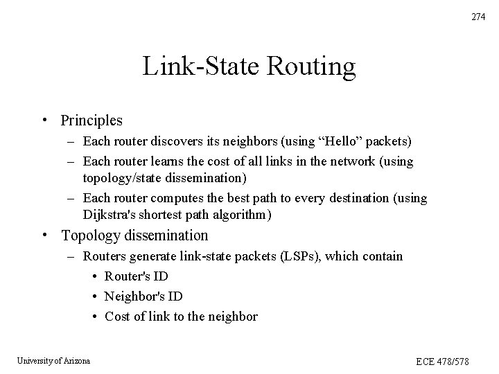
274 Link-State Routing • Principles – Each router discovers its neighbors (using “Hello” packets) – Each router learns the cost of all links in the network (using topology/state dissemination) – Each router computes the best path to every destination (using Dijkstra's shortest path algorithm) • Topology dissemination – Routers generate link-state packets (LSPs), which contain • Router's ID • Neighbor's ID • Cost of link to the neighbor University of Arizona ECE 478/578

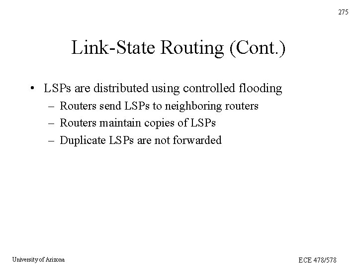
275 Link-State Routing (Cont. ) • LSPs are distributed using controlled flooding – Routers send LSPs to neighboring routers – Routers maintain copies of LSPs – Duplicate LSPs are not forwarded University of Arizona ECE 478/578

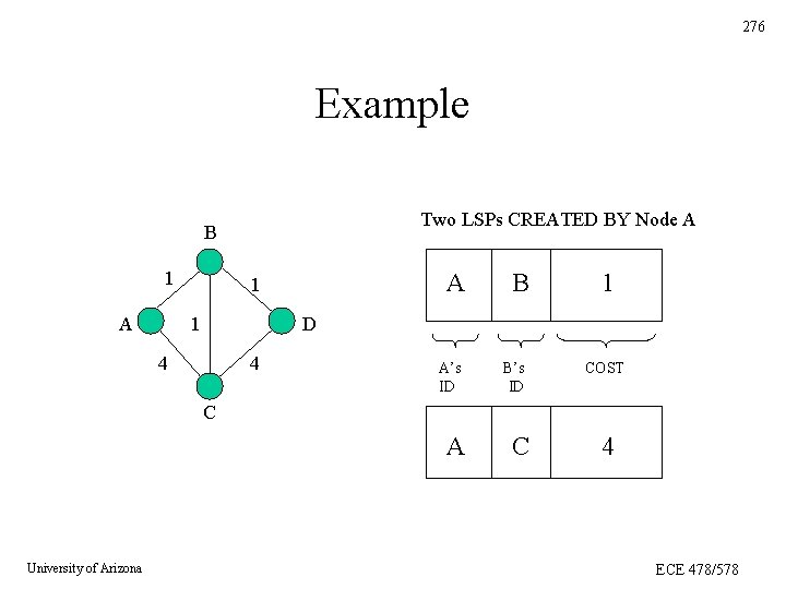
276 Example Two LSPs CREATED BY Node A B 1 A A 1 1 B 1 D 4 4 A’s ID B’s ID COST C A University of Arizona C 4 ECE 478/578

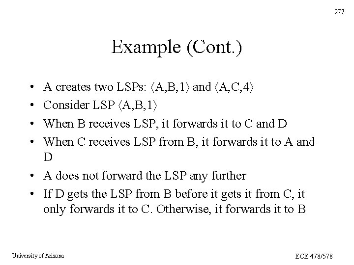
277 Example (Cont. ) A creates two LSPs: A, B, 1 and A, C, 4 Consider LSP A, B, 1 When B receives LSP, it forwards it to C and D When C receives LSP from B, it forwards it to A and D • A does not forward the LSP any further • If D gets the LSP from B before it gets it from C, it only forwards it to C. Otherwise, it forwards it to B • • University of Arizona ECE 478/578

278 Sequence Numbers in Topology Dissemination • LSP consistency problem when a link/router goes down • Solution: use a sequence number for every LSP • LSP with a higher sequence number overwrites an LSP with lower number • Wrap-around problem University of Arizona ECE 478/578

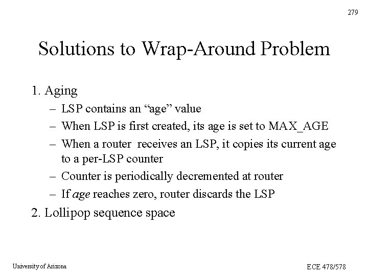
279 Solutions to Wrap-Around Problem 1. Aging – LSP contains an “age” value – When LSP is first created, its age is set to MAX_AGE – When a router receives an LSP, it copies its current age to a per-LSP counter – Counter is periodically decremented at router – If age reaches zero, router discards the LSP 2. Lollipop sequence space University of Arizona ECE 478/578

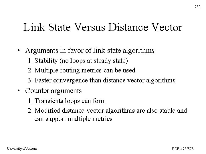
280 Link State Versus Distance Vector • Arguments in favor of link-state algorithms 1. Stability (no loops at steady state) 2. Multiple routing metrics can be used 3. Faster convergence than distance vector algorithms • Counter arguments 1. Transients loops can form 2. Modified distance-vector algorithms are also stable and can support multiple metrics University of Arizona ECE 478/578

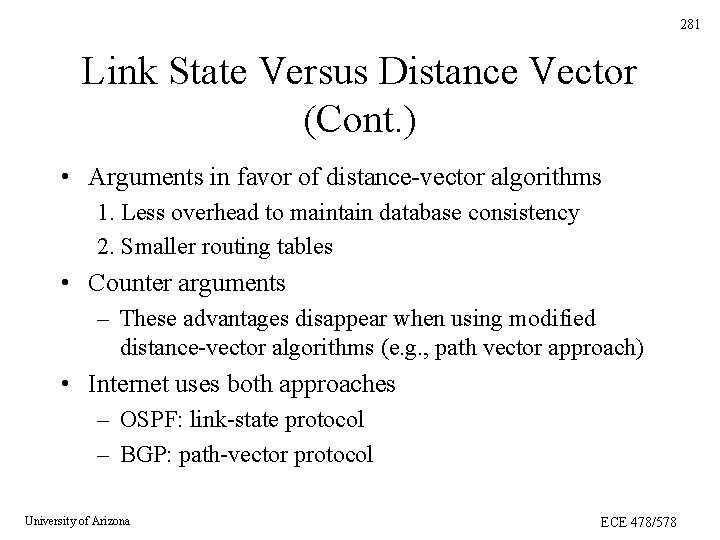
281 Link State Versus Distance Vector (Cont. ) • Arguments in favor of distance-vector algorithms 1. Less overhead to maintain database consistency 2. Smaller routing tables • Counter arguments – These advantages disappear when using modified distance-vector algorithms (e. g. , path vector approach) • Internet uses both approaches – OSPF: link-state protocol – BGP: path-vector protocol University of Arizona ECE 478/578

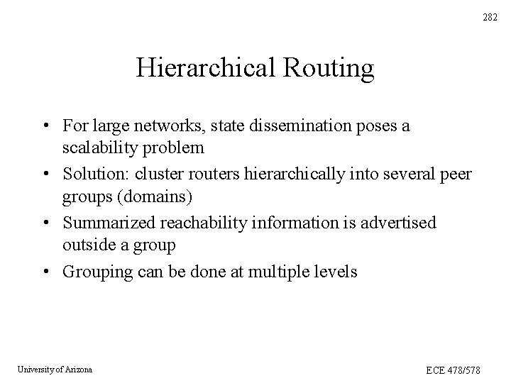
282 Hierarchical Routing • For large networks, state dissemination poses a scalability problem • Solution: cluster routers hierarchically into several peer groups (domains) • Summarized reachability information is advertised outside a group • Grouping can be done at multiple levels University of Arizona ECE 478/578

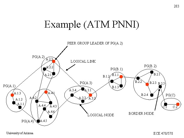
283 Example (ATM PNNI) PEER GROUP LEADER OF PG(A. 2) A. 2. 3 LOGICAL LINK A. 2. 2 A. 2. 1 PG(A. 1) A. 4. 1 A. 1. 2 A. 1. 1 A. 4. 2 B. 2. 2 University of Arizona A. 3. 1 B. 2. 3 B. 2. 5 B. 1. 3 B. 2. 4 PG(C) A. 4. 3 A. 4. 6 PG(A. 4) A. 3. 4 A. 3. 3 A. 3. 2 A. 4. 4 B. 2. 1 B. 1. 2 B. 1. 1 PG(A. 3) A. 1. 3 PG(B. 2) PG(B. 1) C. 1 LOGICAL NODE BORDER NODE A. 4. 5 ECE 478/578 C. 2

284 Traffic Management & Control • Goals: – Guarantee applications Qo. S requirements – Provide congestion control – Utilize resources efficiently • Above goals sometimes conflict with each other • Common approach to traffic management: – Map applications Qo. S into few service classes – Guarantee Qo. S associated with these classes University of Arizona ECE 478/578

285 How Many Classes of Service? • One class – Based on the most demanding traffic – Simple traffic management – Poor bandwidth utilization • Many classes – Better utilization – Traffic management is more complicated University of Arizona ECE 478/578

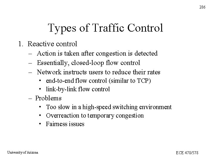
286 Types of Traffic Control 1. Reactive control – Action is taken after congestion is detected – Essentially, closed-loop flow control – Network instructs users to reduce their rates • end-to-end flow control (similar to TCP) • link-by-link flow control – Problems • Too slow in a high-speed switching environment • Overreaction to temporary congestion • Fairness issues University of Arizona ECE 478/578

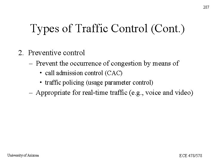
287 Types of Traffic Control (Cont. ) 2. Preventive control – Prevent the occurrence of congestion by means of • call admission control (CAC) • traffic policing (usage parameter control) – Appropriate for real-time traffic (e. g. , voice and video) University of Arizona ECE 478/578

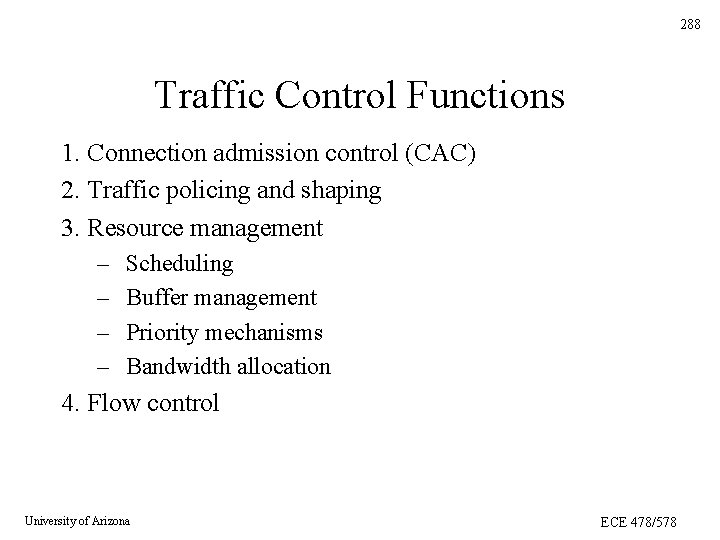
288 Traffic Control Functions 1. Connection admission control (CAC) 2. Traffic policing and shaping 3. Resource management – – Scheduling Buffer management Priority mechanisms Bandwidth allocation 4. Flow control University of Arizona ECE 478/578

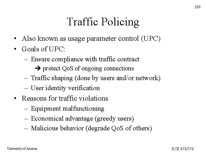
289 Traffic Policing • Also known as usage parameter control (UPC) • Goals of UPC: – Ensure compliance with traffic contract protect Qo. S of ongoing connections – Traffic shaping (done by users and/or network) – User identity verification • Reasons for traffic violations: – Equipment malfunctioning – Economical advantage (greedy users) – Malicious behavior (degrade Qo. S of others) University of Arizona ECE 478/578

290 Traffic Policing (Cont. ) • Several levels of policing (VC, link, etc. ) • Actions taken when violations are detected – Packet discarding, or – Packet tagging (marking packets with lower priority) • Other possible actions at the connection level – Punitive charging – Connection termination – Problems with connection-level actions • long reaction time • drastic penalty University of Arizona ECE 478/578

291 Traffic Policing (Cont. ) • Locations at which traffic policing takes place – Entry nodes (network side of user-network interface) – Boundaries between different networks • Commonly policed parameters: 1. Peak cell rate (PCR) 2. Sustained cell rate (SCR) 3. Maximum burst size (MBS) University of Arizona ECE 478/578

292 Issues in Traffic Policing • Limitations of current set of traffic parameters • How do users estimate their traffic parameters? • Traffic parameters may change within CPE before reaching the policing function tolerance levels are needed University of Arizona ECE 478/578

293 Ideal Requirements in a Policing Mechanism • • Availability Online operation High probability of detecting violations Transparency to conforming connections very low probability of a wrong decision • Short reaction time University of Arizona ECE 478/578

294 Traffic Descriptor • Set of traffic parameters describing a source • Used as basis for traffic contract • Often based on a traffic envelope – – Time-invariant bound on number of arrivals Often, it represents the worst-case (deterministic) behavior Also known as “traffic constraint function” Examples: • peak rate • ( , ) model • linear bounded arrival processes (LBAP) University of Arizona ECE 478/578

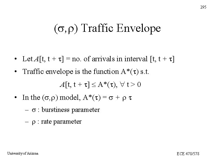
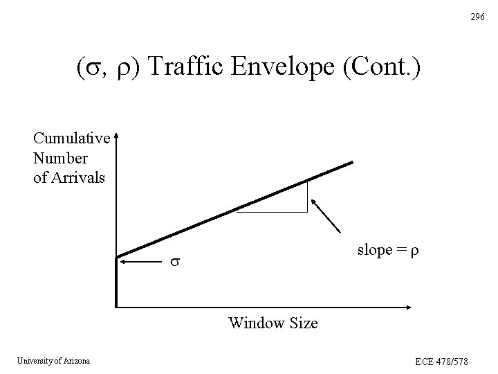
295 ( , ) Traffic Envelope • Let A[t, t + ] = no. of arrivals in interval [t, t + ] • Traffic envelope is the function A*( ) s. t. A[t, t + ] A*( ), t > 0 • In the ( , ) model, A*( ) = + – : burstiness parameter – : rate parameter University of Arizona ECE 478/578

296 ( , ) Traffic Envelope (Cont. ) Cumulative Number of Arrivals slope = Window Size University of Arizona ECE 478/578

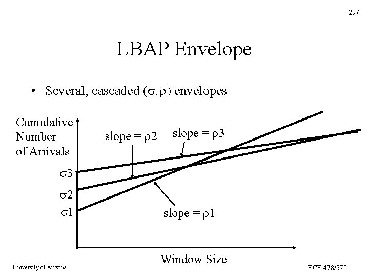
297 LBAP Envelope • Several, cascaded ( , ) envelopes Cumulative Number of Arrivals slope = 2 slope = 3 3 2 1 University of Arizona slope = 1 Window Size ECE 478/578

298 Properties of a good traffic descriptor 1. Representativity 2. Verifiability 3. Preservability 4. Usability University of Arizona ECE 478/578

299 Common Policing Mechanisms 1. Leaky bucket 2. Jumping window 3. Moving window 4. Triggered jumping window 5. Exponentially weighted moving average University of Arizona ECE 478/578

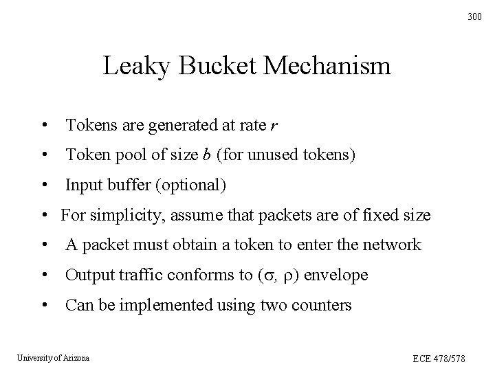
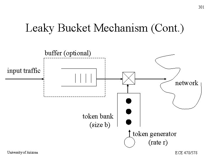
300 Leaky Bucket Mechanism • Tokens are generated at rate r • Token pool of size b (for unused tokens) • Input buffer (optional) • For simplicity, assume that packets are of fixed size • A packet must obtain a token to enter the network • Output traffic conforms to ( , ) envelope • Can be implemented using two counters University of Arizona ECE 478/578

301 Leaky Bucket Mechanism (Cont. ) buffer (optional) input traffic network token bank (size b) token generator (rate r) University of Arizona ECE 478/578

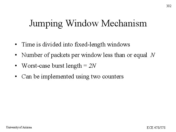
302 Jumping Window Mechanism • Time is divided into fixed-length windows • Number of packets per window less than or equal N • Worst-case burst length = 2 N • Can be implemented using two counters University of Arizona ECE 478/578

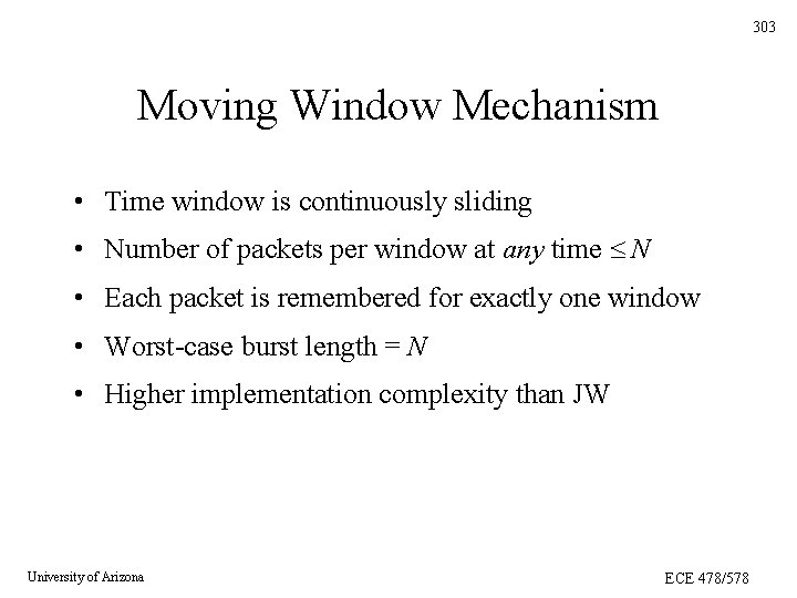
303 Moving Window Mechanism • Time window is continuously sliding • Number of packets per window at any time N • Each packet is remembered for exactly one window • Worst-case burst length = N • Higher implementation complexity than JW University of Arizona ECE 478/578

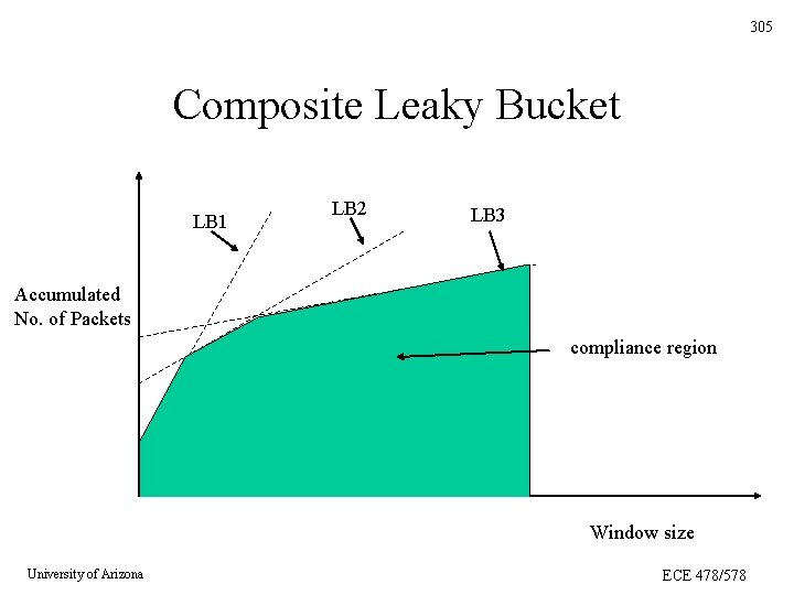
304 Composite Policing Mechanisms • Previous mechanisms enforce simple envelopes • To enforce more representative traffic envelopes, composite policing mechanisms can be used • A composite mechanism consists of several basic policing mechanisms connected in cascade • Example: Composite Leaky Bucket (i. e. , LBAP) University of Arizona ECE 478/578

305 Composite Leaky Bucket LB 1 LB 2 LB 3 Accumulated No. of Packets compliance region Window size University of Arizona ECE 478/578

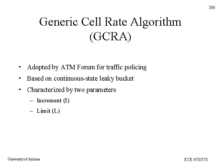
306 Generic Cell Rate Algorithm (GCRA) • Adopted by ATM Forum for traffic policing • Based on continuous-state leaky bucket • Characterized by two parameters – Increment (I) – Limit (L) University of Arizona ECE 478/578

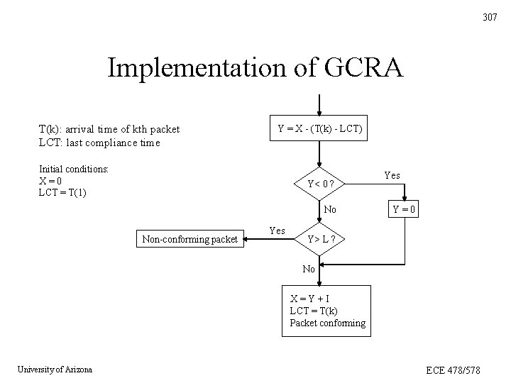
307 Implementation of GCRA T(k): arrival time of kth packet LCT: last compliance time Y = X - (T(k) - LCT) Initial conditions: X=0 LCT = T(1) Y< 0 ? No Non-conforming packet Yes Y=0 Y> L ? No X=Y+I LCT = T(k) Packet conforming University of Arizona ECE 478/578

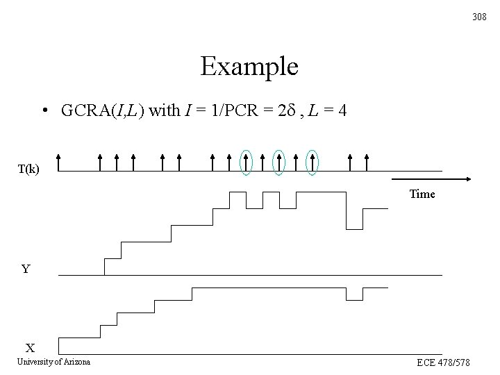
308 Example • GCRA(I, L) with I = 1/PCR = 2 , L = 4 T(k) Time Y X University of Arizona ECE 478/578