240 373 Image Processing Montri Karnjanadecha montricoe psu
- Slides: 39

240 -373 Image Processing Montri Karnjanadecha montri@coe. psu. ac. th http: //fivedots. coe. psu. ac. th/~montri 240 -373: Chapter 12: Image Compression 1

Chapter 12 Image Compression 240 -373: Chapter 12: Image Compression 2

Image Compression • Purposes – To minimize storage space – To maximize transfer speed – To minimize hardware costs • Requirements – – Speedy operation (compression and unpacking( Significantly reduction in required memory No significant loss of quality Format of output suitable for transfer and storage 240 -373: Chapter 12: Image Compression 3

Image Compression • Types – Statistical compression--based on pixels in whole image – Spatial compression--based on the spatial relationship of pixels of similar type – Quantizing compression--reducing number of gray levels and resolution – Fractal compression--based on fractal generating functions 240 -373: Chapter 12: Image Compression 4

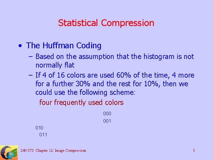
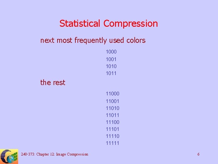
Statistical Compression • The Huffman Coding – Based on the assumption that the histogram is not normally flat – If 4 of 16 colors are used 60% of the time, 4 more for a further 30% and the rest for 10%, then we could use the following scheme: four frequently used colors 000 001 010 011 240 -373: Chapter 12: Image Compression 5

Statistical Compression next most frequently used colors 1000 1001 1010 1011 the rest 11000 11001 11010 11011 11100 11101 11110 11111 240 -373: Chapter 12: Image Compression 6

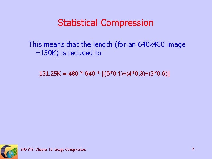
Statistical Compression This means that the length (for an 640 x 480 image =150 K) is reduced to 131. 25 K = 480 * 640 * [(5*0. 1)+(4*0. 3)+(3*0. 6)] 240 -373: Chapter 12: Image Compression 7

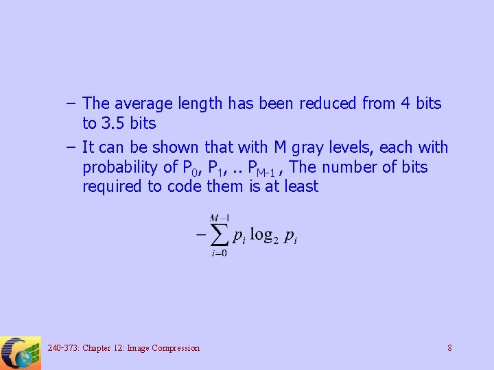
– The average length has been reduced from 4 bits to 3. 5 bits – It can be shown that with M gray levels, each with probability of P 0, P 1, . . PM-1 , The number of bits required to code them is at least 240 -373: Chapter 12: Image Compression 8

Huffman Coding Technique 1: The Huffman Code USE: To reduce the space that an image uses on disk or in transit OPERATION: – Order the gray levels according to their frequency of use, most occurrence first – Combine the two least used gray levels into one group, combine their frequencies and reorder the gray levels 240 -373: Chapter 12: Image Compression 9

Huffman Coding OPERATION: (cont’d( – Continue to do this until only two gray levels are left – Now allocate a 0 to one of these gray-level groups and a 1 to the other – Work back through the groupings so that where two groups have been combined to form a new, larger, group which is currently coded as ‘ccc’ – Code one of the smaller groups as ccc 0 and the other as ccc 1 240 -373: Chapter 12: Image Compression 10

Huffman coding example • Example: For a nine-color system, we obtain the following coding: 01 5100000 0 000 610001 1 1001 7101 2 100001 8001 3 11 5 Storage has improved from 19000*3 bits (57000) to 51910 bits. 240 -373: Chapter 12: Image Compression 11

240 -373: Chapter 12: Image Compression 12

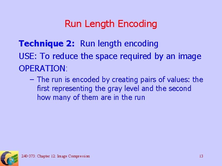
Run Length Encoding Technique 2: Run length encoding USE: To reduce the space required by an image OPERATION: – The run is encoded by creating pairs of values: the first representing the gray level and the second how many of them are in the run 240 -373: Chapter 12: Image Compression 13

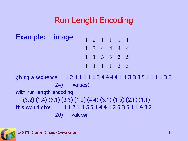
Run Length Encoding Example: image giving a sequence: 1 2 1 1 1 3 4 4 1 1 3 3 3 5 1 1 3 3 24) values( with run length encoding (3, 2) (1, 4) (5, 1) (3, 3) (1, 2) (4, 4) (3, 1) (1, 5) (2, 1) (1, 1) this would give: 11211531441233511432 20) values( 240 -373: Chapter 12: Image Compression 14

Run Length Encoding • Notes – Huffman coding can be performed after Run length encoding – It might be possible to implement the Huffman code only on the run lengths 240 -373: Chapter 12: Image Compression 15

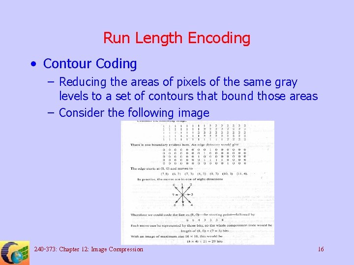
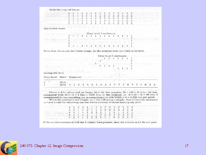
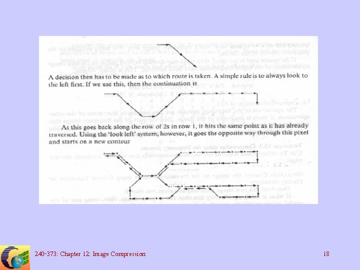
Run Length Encoding • Contour Coding – Reducing the areas of pixels of the same gray levels to a set of contours that bound those areas – Consider the following image 240 -373: Chapter 12: Image Compression 16

240 -373: Chapter 12: Image Compression 17

240 -373: Chapter 12: Image Compression 18

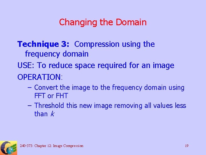
Changing the Domain Technique 3: Compression using the frequency domain USE: To reduce space required for an image OPERATION: – Convert the image to the frequency domain using FFT or FHT – Threshold this new image removing all values less than k 240 -373: Chapter 12: Image Compression 19

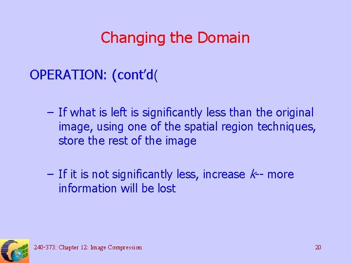
Changing the Domain OPERATION: (cont’d( – If what is left is significantly less than the original image, using one of the spatial region techniques, store the rest of the image – If it is not significantly less, increase k-- more information will be lost 240 -373: Chapter 12: Image Compression 20

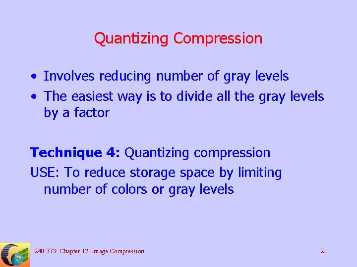
Quantizing Compression • Involves reducing number of gray levels • The easiest way is to divide all the gray levels by a factor Technique 4: Quantizing compression USE: To reduce storage space by limiting number of colors or gray levels 240 -373: Chapter 12: Image Compression 21

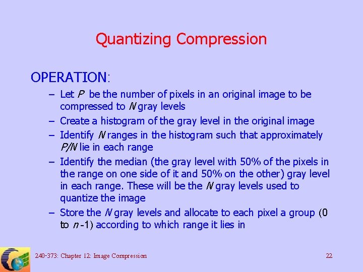
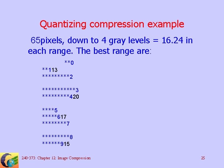
Quantizing Compression OPERATION: – Let P be the number of pixels in an original image to be compressed to N gray levels – Create a histogram of the gray level in the original image – Identify N ranges in the histogram such that approximately P/N lie in each range – Identify the median (the gray level with 50% of the pixels in the range on one side of it and 50% on the other) gray level in each range. These will be the N gray levels used to quantize the image – Store the N gray levels and allocate to each pixel a group (0 to n -1) according to which range it lies in 240 -373: Chapter 12: Image Compression 22

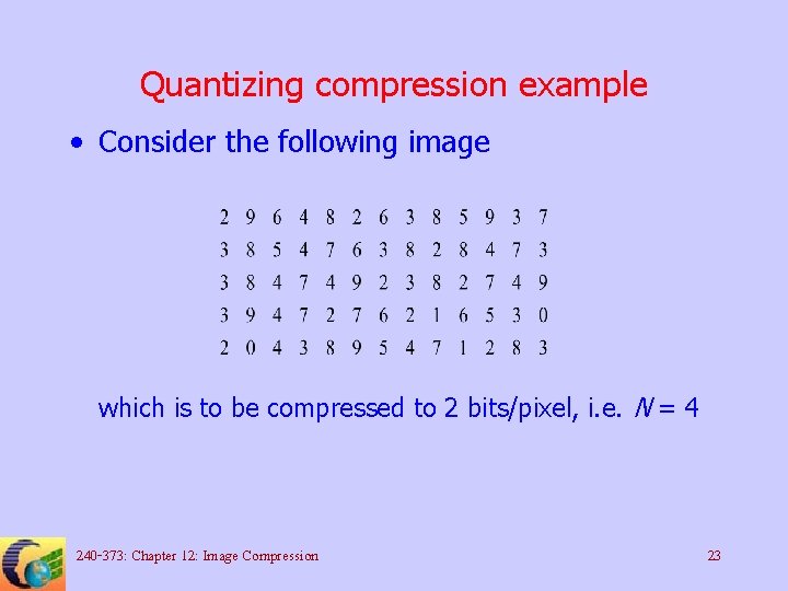
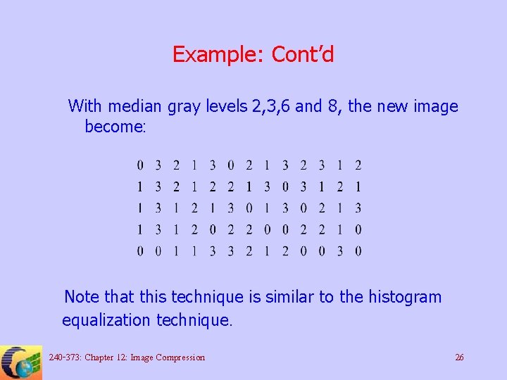
Quantizing compression example • Consider the following image which is to be compressed to 2 bits/pixel, i. e. N = 4 240 -373: Chapter 12: Image Compression 23

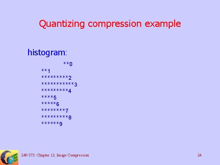
Quantizing compression example histogram: **0 **1 *****2 ******3 *****4 ****5 *****6 ****7 *****8 ******9 240 -373: Chapter 12: Image Compression 24

Quantizing compression example 65 pixels, down to 4 gray levels = 16. 24 in each range. The best range are: **0 **113 *****2 ******3 *****420 ****5 *****617 *********8 ******915 240 -373: Chapter 12: Image Compression 25

Example: Cont’d With median gray levels 2, 3, 6 and 8, the new image become: Note that this technique is similar to the histogram equalization technique. 240 -373: Chapter 12: Image Compression 26

Fractal Compression • Fractal Compression – Yields 10000: 1 compression ratio – Can also yield 1000000: 1 compression ration with conventional algorithm added – Based on very simple functions to generate (in multi-dimensional space) highly complex and totally predictable pattern – Fractal graphics workstations: a 640 x 480 VGA image requires 5800 bytes of storage 240 -373: Chapter 12: Image Compression 27

Real-Time Image Transmission • Compressing and sending a sequence of images in real-time • Most of real-time vision systems send many images of the same type before changing the image to a new scene • For example, most television program will dwell on a scene for at least 5 seconds 240 -373: Chapter 12: Image Compression 28

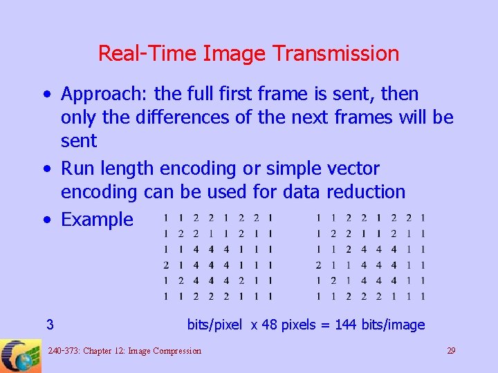
Real-Time Image Transmission • Approach: the full first frame is sent, then only the differences of the next frames will be sent • Run length encoding or simple vector encoding can be used for data reduction • Example 3 bits/pixel x 48 pixels = 144 bits/image 240 -373: Chapter 12: Image Compression 29

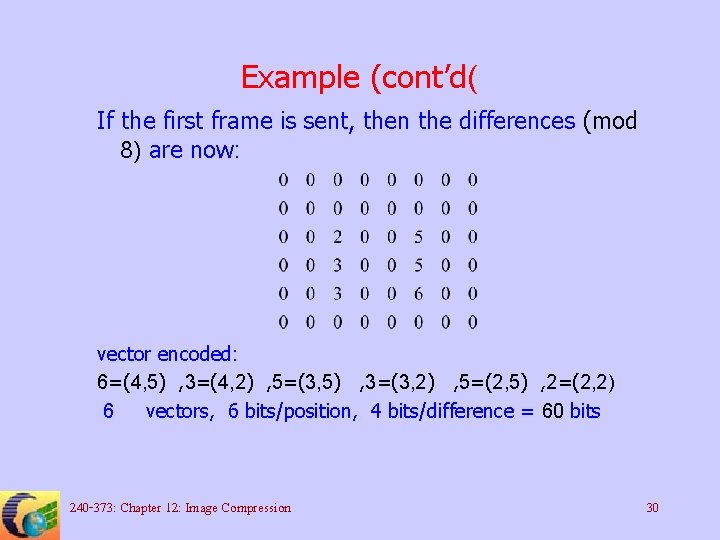
Example (cont’d( If the first frame is sent, then the differences (mod 8) are now: vector encoded: 6=(4, 5) , 3=(4, 2) , 5=(3, 5) , 3=(3, 2) , 5=(2, 5) , 2=(2, 2) 6 vectors, 6 bits/position, 4 bits/difference = 60 bits 240 -373: Chapter 12: Image Compression 30

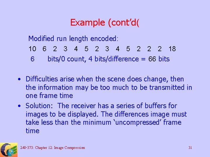
Example (cont’d( Modified run length encoded: 10 6 2 3 4 5 2 2 2 18 6 bits/0 count, 4 bits/difference = 66 bits • Difficulties arise when the scene does change, then the information may be too much to be transmitted in one frame time • Solution: The receiver has a series of buffers for images to be displayed. The differences image must take less than the minimum ‘uncompressed’ frame time 240 -373: Chapter 12: Image Compression 31

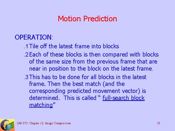
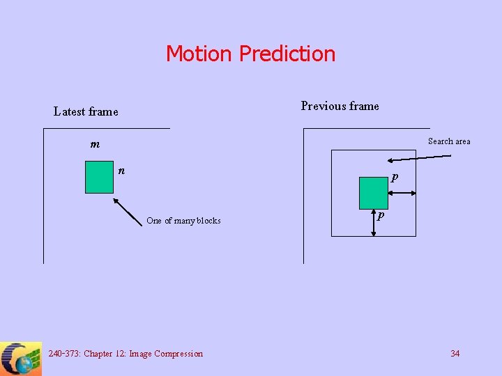
Motion Prediction • The image may still have the same constituent parts but they may have all shifted in one direction Technique 5: Block matching for motion prediction USE: Saving space by estimating what motion has occurred between past and present images, then only saving the changes. 240 -373: Chapter 12: Image Compression 32

Motion Prediction OPERATION: . 1 Tile off the latest frame into blocks. 2 Each of these blocks is then compared with blocks of the same size from the previous frame that are near in position to the block on the latest frame. . 3 This has to be done for all blocks in the latest frame. Then the best match (and the corresponding predicted movement vector) is determined. This is called “ full-search block matching” 240 -373: Chapter 12: Image Compression 33

Motion Prediction Previous frame Latest frame m Search area n p One of many blocks 240 -373: Chapter 12: Image Compression p 34

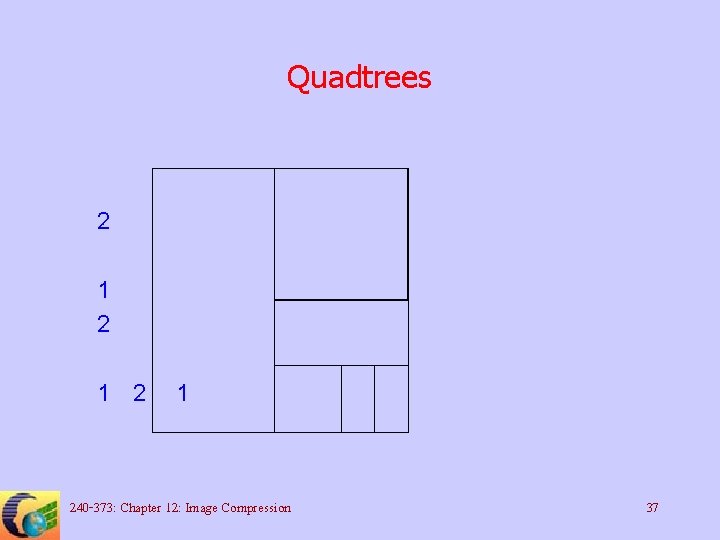
Quadtrees • A quadtree is a recursive segmenting of an image into four parts • A suitable compression method for an image that has large area of the same colored pixels and rectangular in character 240 -373: Chapter 12: Image Compression 35

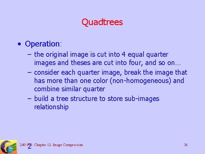
Quadtrees • Operation: – the original image is cut into 4 equal quarter images and theses are cut into four, and so on… – consider each quarter image, break the image that has more than one color (non-homogeneous) and combine similar quarter – build a tree structure to store sub-images relationship 240 -373: 2 Chapter 12: Image Compression 36

Quadtrees 2 1 2 1 240 -373: Chapter 12: Image Compression 37

Standard Image File Format – – – – . BMP. PIC. PCX. PIG. TIFF. GIF. JPG etc. 240 -373: Chapter 12: Image Compression 38

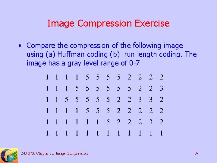
Image Compression Exercise • Compare the compression of the following image using (a) Huffman coding (b) run length coding. The image has a gray level range of 0 -7. 240 -373: Chapter 12: Image Compression 39