2020116 CV Motion 2 2020116 CV Motion 4

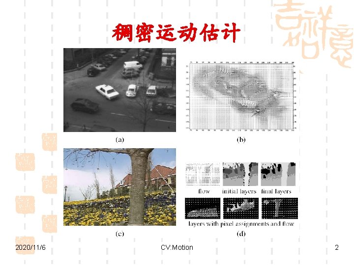
稠密运动估计 2020/11/6 CV: Motion 2

2020/11/6 CV: Motion 4

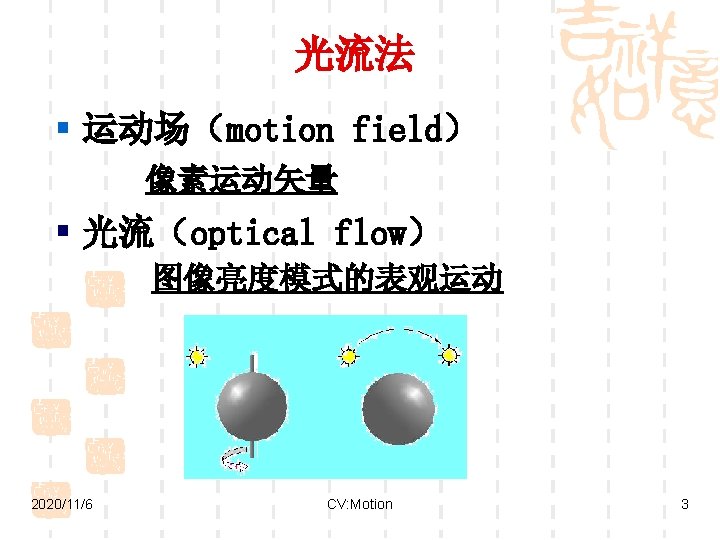
8. 1 二维光流运动估计 § 根据图像亮度模式的变化估计物体的 运动 1. 基于梯度的方法 (Gradientbased) Differential Methods 2. 块匹配方法 (Block Matching) Region Matching 2020/11/6 CV: Motion 5

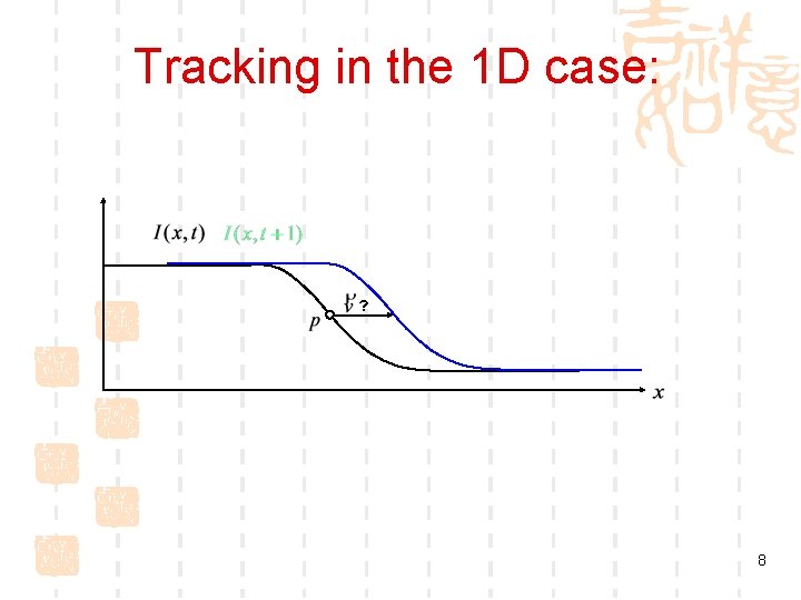
Tracking in the 1 D case: ? 8

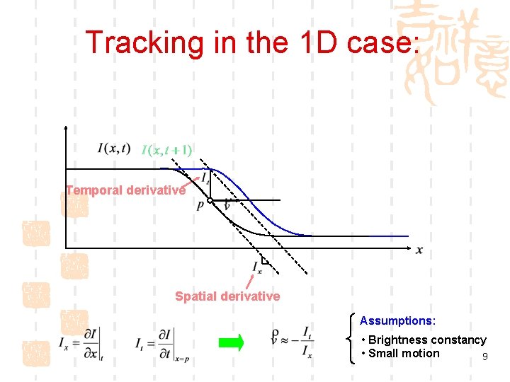
Tracking in the 1 D case: Temporal derivative Spatial derivative Assumptions: • Brightness constancy • Small motion 9

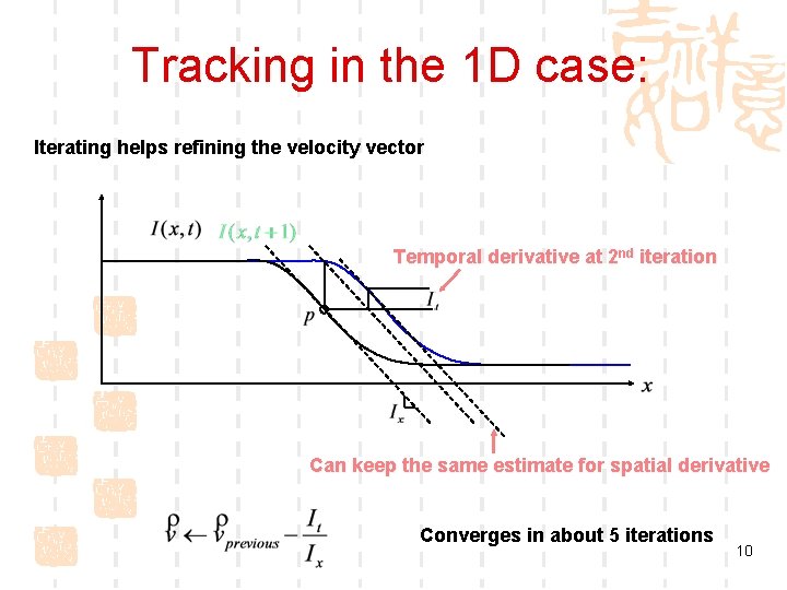
Tracking in the 1 D case: Iterating helps refining the velocity vector Temporal derivative at 2 nd iteration Can keep the same estimate for spatial derivative Converges in about 5 iterations 10

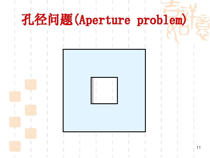
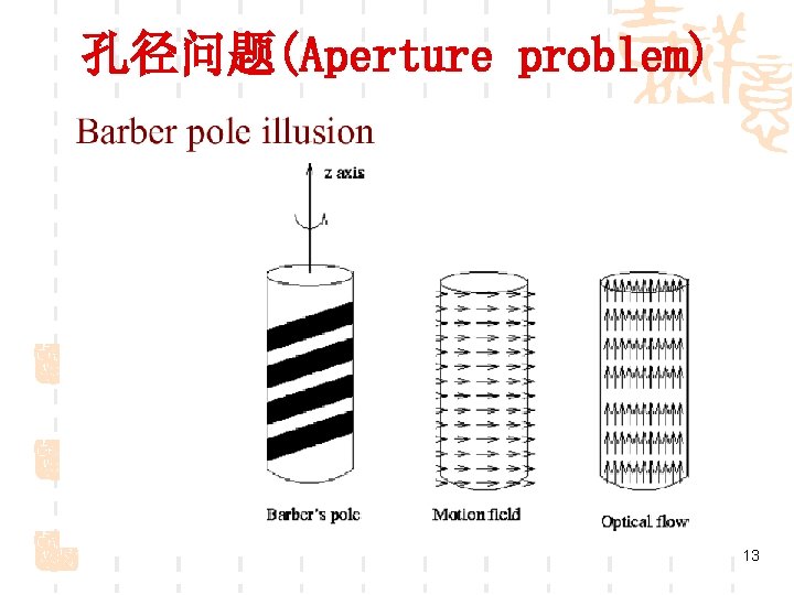
孔径问题(Aperture problem) 11

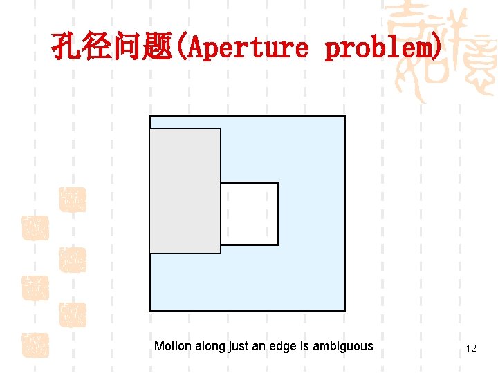
孔径问题(Aperture problem) Motion along just an edge is ambiguous 12

孔径问题(Aperture problem) 13

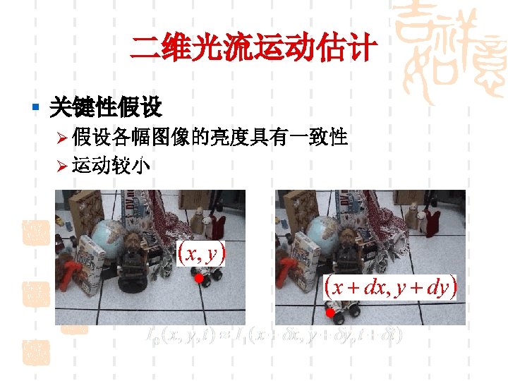
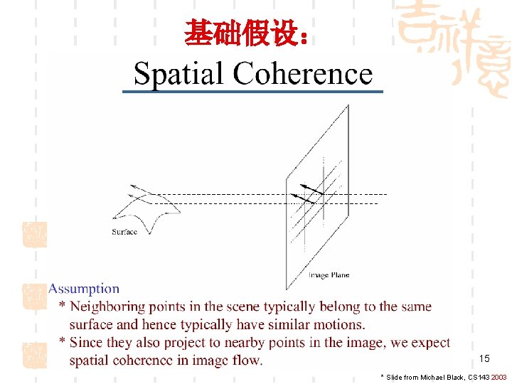
基础假设： 15 * Slide from Michael Black, CS 143 2003

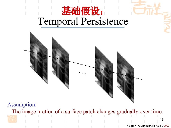
基础假设： 16 * Slide from Michael Black, CS 143 2003

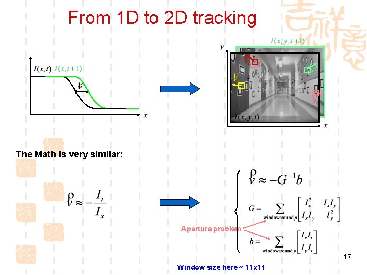
From 1 D to 2 D tracking The Math is very similar: Aperture problem 17 Window size here ~ 11 x 11

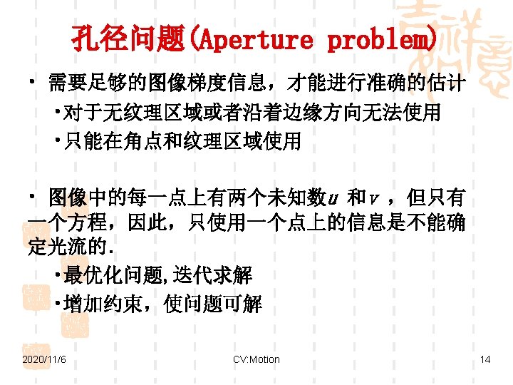
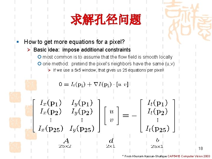
求解孔径问题 § How to get more equations for a pixel? Ø Basic idea: impose additional constraints ¡ most common is to assume that the flow field is smooth locally ¡ one method: pretend the pixel’s neighbors have the same (u, v) Ø If we use a 5 x 5 window, that gives us 25 equations per pixel! 18 * From Khurram Hassan-Shafique CAP 5415 Computer Vision 2003

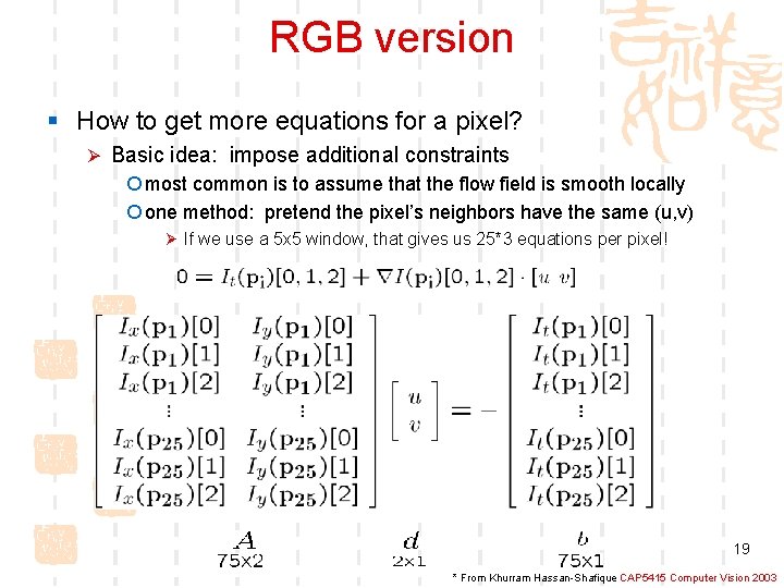
RGB version § How to get more equations for a pixel? Ø Basic idea: impose additional constraints ¡ most common is to assume that the flow field is smooth locally ¡ one method: pretend the pixel’s neighbors have the same (u, v) Ø If we use a 5 x 5 window, that gives us 25*3 equations per pixel! 19 * From Khurram Hassan-Shafique CAP 5415 Computer Vision 2003

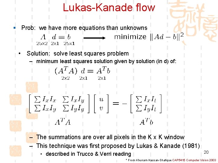
Lukas-Kanade flow § Prob: we have more equations than unknowns • Solution: solve least squares problem – minimum least squares solution given by solution (in d) of: – The summations are over all pixels in the K x K window – This technique was first proposed by Lukas & Kanade (1981) • described in Trucco & Verri reading 20 * From Khurram Hassan-Shafique CAP 5415 Computer Vision 2003

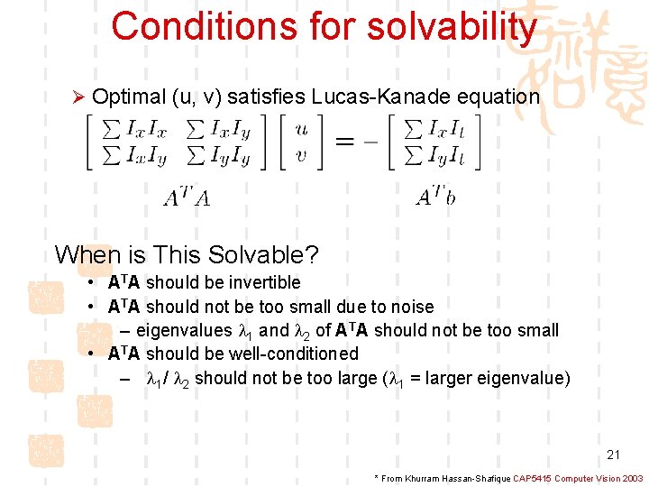
Conditions for solvability Ø Optimal (u, v) satisfies Lucas-Kanade equation When is This Solvable? • ATA should be invertible • ATA should not be too small due to noise – eigenvalues l 1 and l 2 of ATA should not be too small • ATA should be well-conditioned – l 1/ l 2 should not be too large (l 1 = larger eigenvalue) 21 * From Khurram Hassan-Shafique CAP 5415 Computer Vision 2003

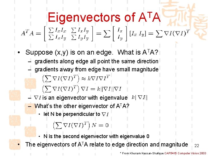
Eigenvectors of ATA • Suppose (x, y) is on an edge. What is ATA? – gradients along edge all point the same direction – gradients away from edge have small magnitude – is an eigenvector with eigenvalue – What’s the other eigenvector of ATA? • let N be perpendicular to • N is the second eigenvector with eigenvalue 0 • The eigenvectors of ATA relate to edge direction and magnitude 22 * From Khurram Hassan-Shafique CAP 5415 Computer Vision 2003

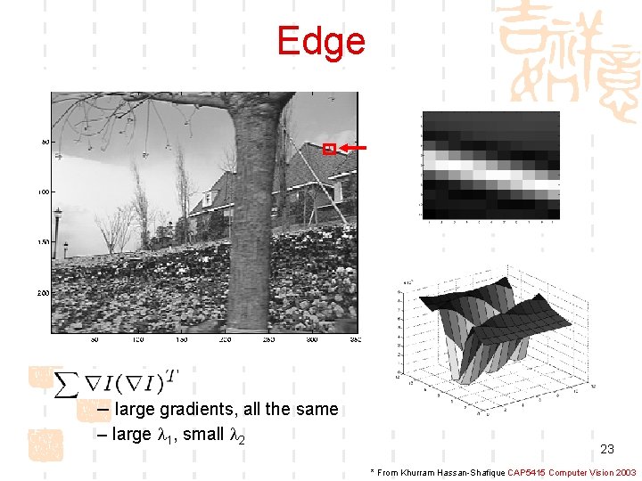
Edge – large gradients, all the same – large l 1, small l 2 23 * From Khurram Hassan-Shafique CAP 5415 Computer Vision 2003

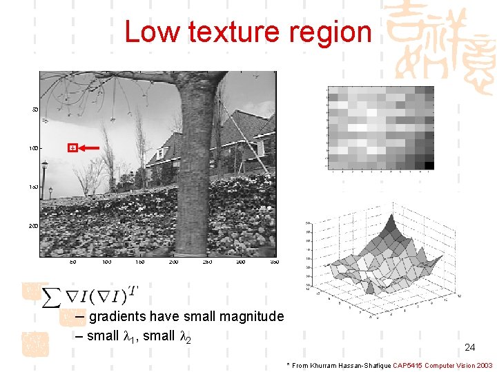
Low texture region – gradients have small magnitude – small l 1, small l 2 24 * From Khurram Hassan-Shafique CAP 5415 Computer Vision 2003

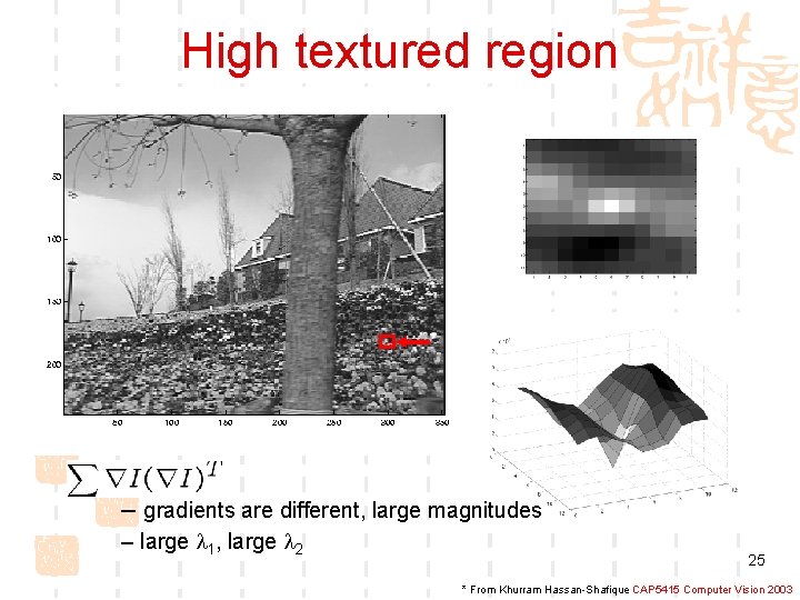
High textured region – gradients are different, large magnitudes – large l 1, large l 2 25 * From Khurram Hassan-Shafique CAP 5415 Computer Vision 2003

Observation § This is a two image problem BUT Ø Can measure sensitivity by just looking at one of the images! Ø This tells us which pixels are easy to track, which are hard ¡ very useful later on when we do feature tracking. . . 26 * From Khurram Hassan-Shafique CAP 5415 Computer Vision 2003

误差分析 What are the potential causes of errors in this procedure? Ø Suppose ATA is easily invertible Ø Suppose there is not much noise in the image • When our assumptions are violated – Brightness constancy is not satisfied – The motion is not small – A point does not move like its neighbors • window size is too large • what is the ideal window size? 27 * From Khurram Hassan-Shafique CAP 5415 Computer Vision 2003

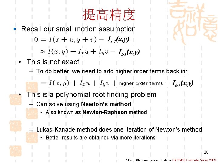
提高精度 § Recall our small motion assumption It-1(x, y) • This is not exact – To do better, we need to add higher order terms back in: It-1(x, y) • This is a polynomial root finding problem – Can solve using Newton’s method • Also known as Newton-Raphson method – Lukas-Kanade method does one iteration of Newton’s method • Better results are obtained via more iterations 28 * From Khurram Hassan-Shafique CAP 5415 Computer Vision 2003

迭代更新 • Iterative Lukas-Kanade Algorithm 1. Estimate velocity at each pixel by solving Lucas. Kanade equations 2. Warp I(t-1) towards I(t) using the estimated flow field - use image warping techniques 3. Repeat until convergence 29 * From Khurram Hassan-Shafique CAP 5415 Computer Vision 2003

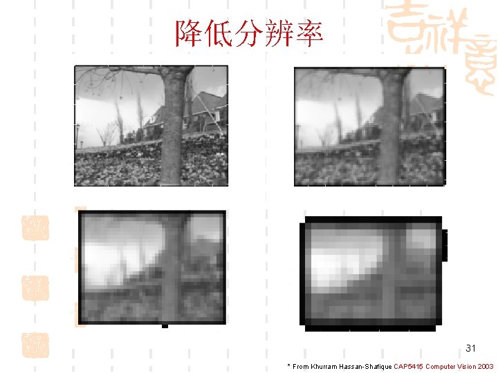
降低分辨率 31 * From Khurram Hassan-Shafique CAP 5415 Computer Vision 2003

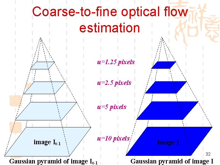
Coarse-to-fine optical flow estimation u=1. 25 pixels u=2. 5 pixels u=5 pixels image It-1 u=10 pixels image I 32 Gaussian pyramid of image It-1 Gaussian pyramid of image I

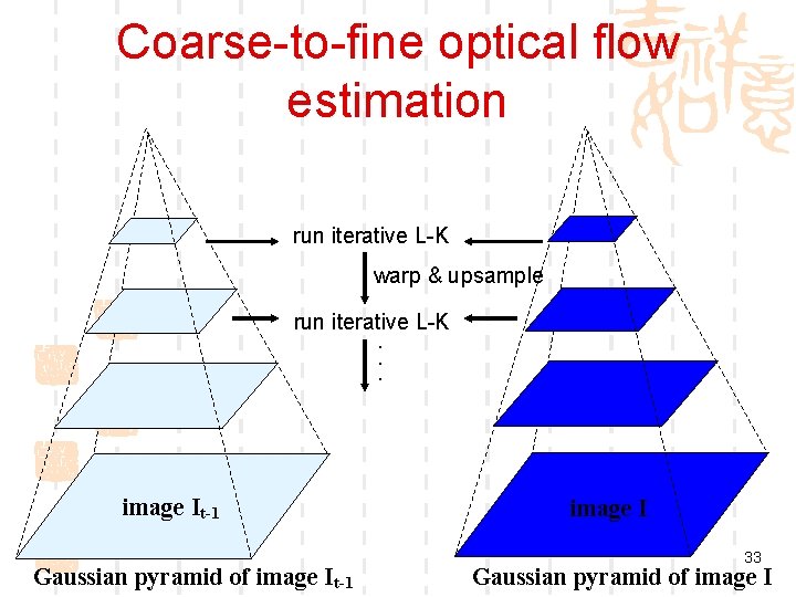
Coarse-to-fine optical flow estimation run iterative L-K warp & upsample run iterative L-K. . . image JIt-1 Gaussian pyramid of image It-1 image I 33 Gaussian pyramid of image I

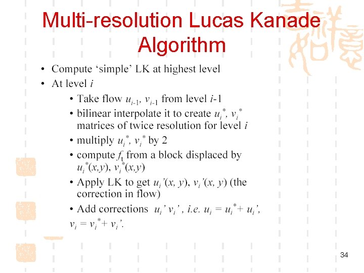
Multi-resolution Lucas Kanade Algorithm 34

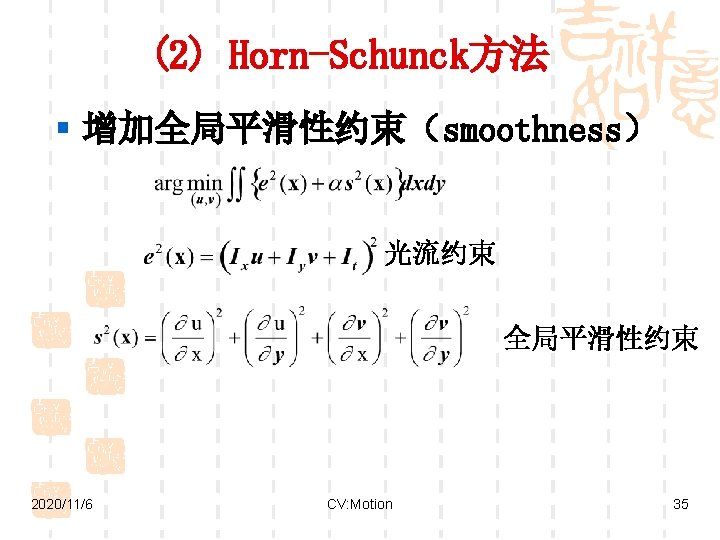
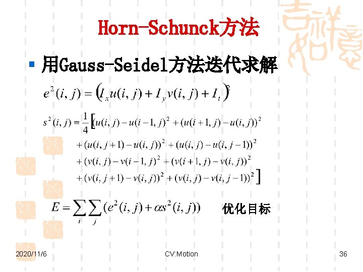
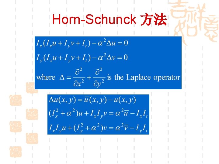
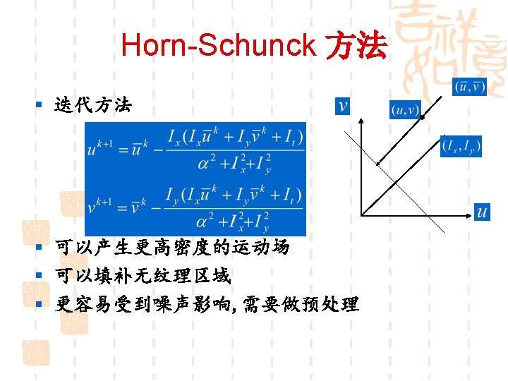
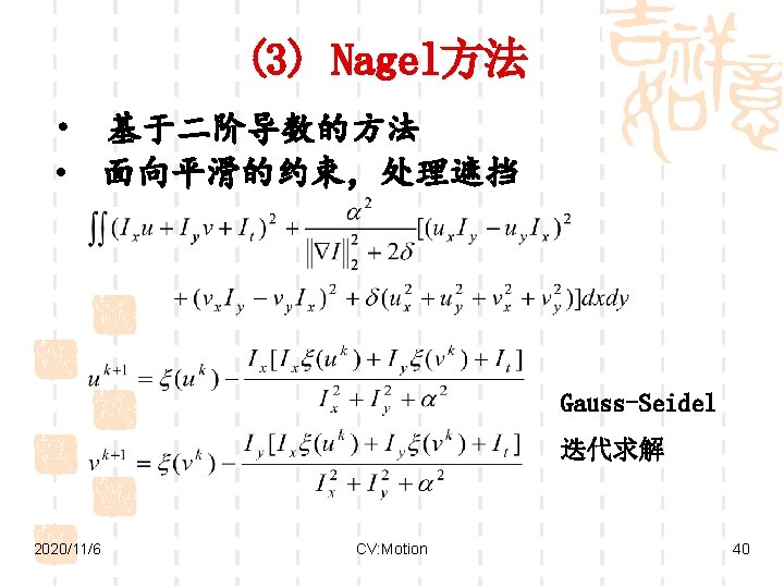
Horn-Schunck方法 § 用Gauss-Seidel方法迭代求解 优化目标 2020/11/6 CV: Motion 36

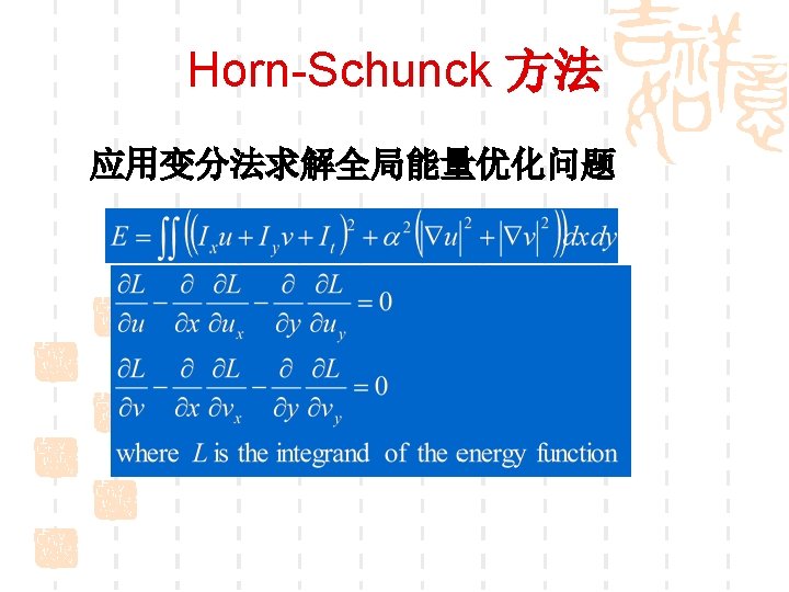
Horn-Schunck 方法

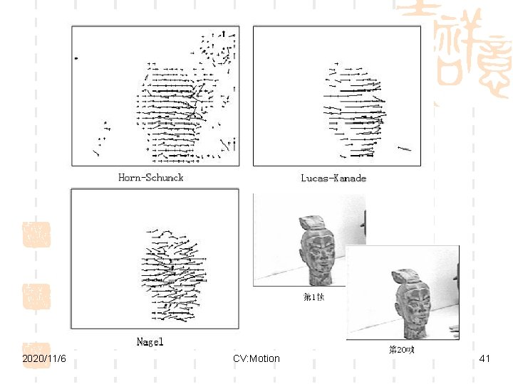
2020/11/6 CV: Motion 41

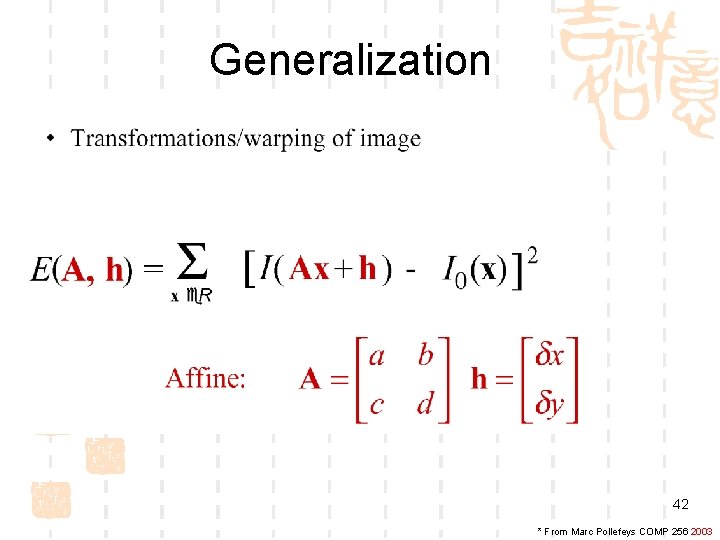
Generalization 42 * From Marc Pollefeys COMP 256 2003

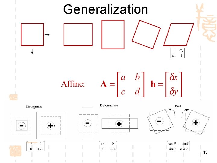
Generalization 43

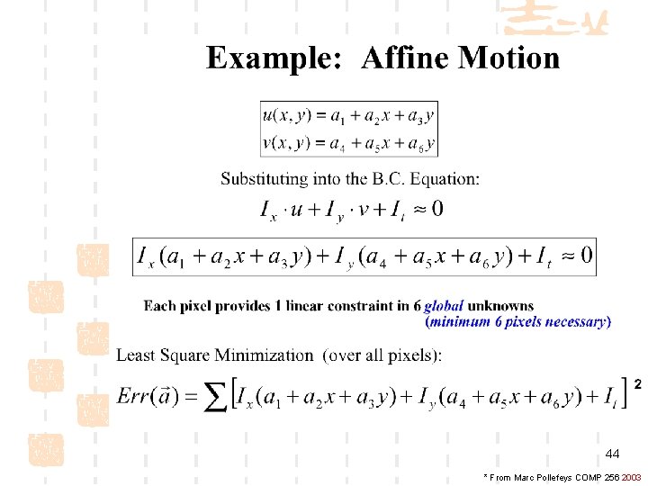
44 * From Marc Pollefeys COMP 256 2003

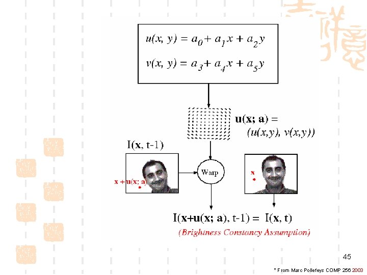
45 * From Marc Pollefeys COMP 256 2003

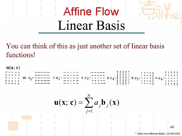
Affine Flow 46 * Slide from Michael Black, CS 143 2003