2013 Cengage Learning All Rights Reserved May not

© 2013 Cengage Learning. All Rights Reserved. May not be copied, scanned, or duplicated, in whole or in part, except for use as permitted in a license distributed with a certain product or service or otherwise on a password-protected website for classroom use.

Chapter 2: Basic Tools for Forecasting 2. 1 Types of data 2. 2 Time series plots 2. 3 Scatterplots 2. 4 Summarizing the data o o 2. 5 2. 6 2. 7 2. 8 2. 9 Measures of average Measures of variation Correlation Transformations How to measure forecasting accuracy Prediction intervals Basic principles 2 © 2013 Cengage Learning. All Rights Reserved. May not be copied, scanned, or duplicated, in whole or in part, except for use as permitted in a license distributed with a certain product or service or otherwise on a password-protected website for classroom use.

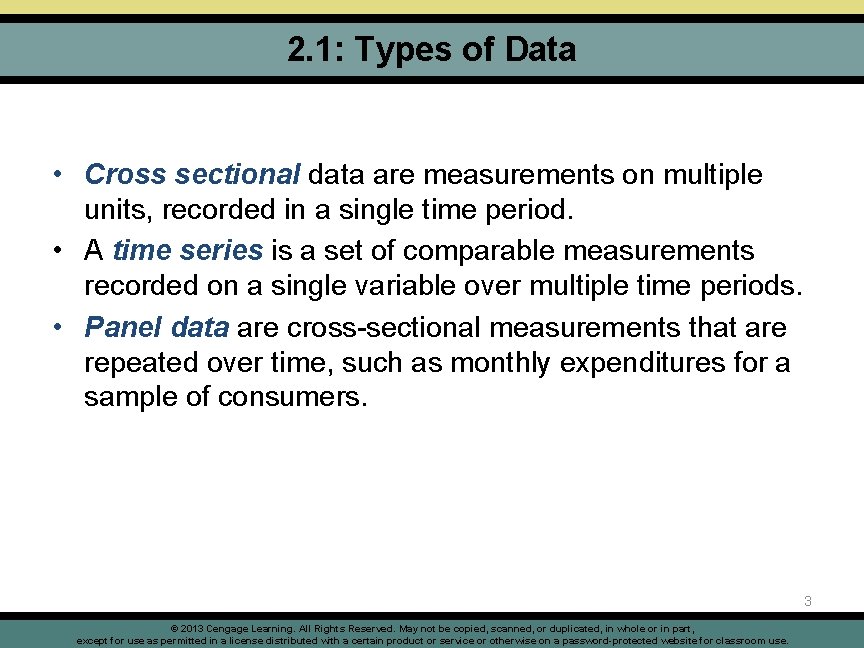
2. 1: Types of Data • Cross sectional data are measurements on multiple units, recorded in a single time period. • A time series is a set of comparable measurements recorded on a single variable over multiple time periods. • Panel data are cross-sectional measurements that are repeated over time, such as monthly expenditures for a sample of consumers. 3 © 2013 Cengage Learning. All Rights Reserved. May not be copied, scanned, or duplicated, in whole or in part, except for use as permitted in a license distributed with a certain product or service or otherwise on a password-protected website for classroom use.

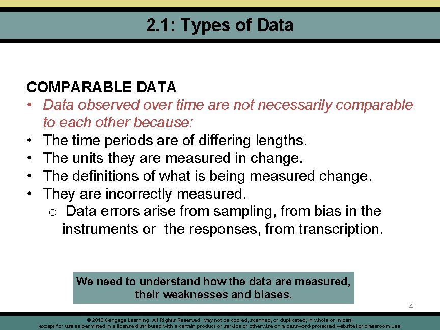
2. 1: Types of Data COMPARABLE DATA • Data observed over time are not necessarily comparable to each other because: • The time periods are of differing lengths. • The units they are measured in change. • The definitions of what is being measured change. • They are incorrectly measured. o Data errors arise from sampling, from bias in the instruments or the responses, from transcription. We need to understand how the data are measured, their weaknesses and biases. 4 © 2013 Cengage Learning. All Rights Reserved. May not be copied, scanned, or duplicated, in whole or in part, except for use as permitted in a license distributed with a certain product or service or otherwise on a password-protected website for classroom use.

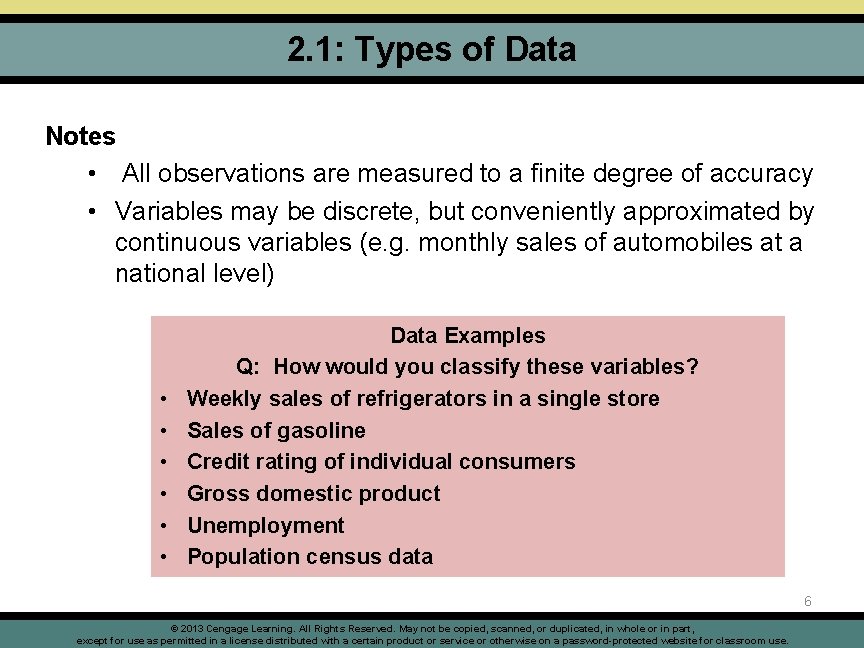
2. 1: Types of Data • Data may be: o Categorical (e. g. industrial classification) o Ordinal (e. g. Bond ratings, AAA, AAa, …) o Interval scaled (e. g. temperature: Fahrenheit or Celsius) o Ratio-scaled (e. g. monthly sales) • Data may be: o Discrete or continuous (e. g. number of commercials shown during a one-hour period vs. time devoted to commercials during that hour) o Time series or cross-sectional (e. g. stock price over time vs. multiple stock prices on a given day o Stock or flow (e. g. capital vs. income) 5 © 2013 Cengage Learning. All Rights Reserved. May not be copied, scanned, or duplicated, in whole or in part, except for use as permitted in a license distributed with a certain product or service or otherwise on a password-protected website for classroom use.

2. 1: Types of Data Notes • All observations are measured to a finite degree of accuracy • Variables may be discrete, but conveniently approximated by continuous variables (e. g. monthly sales of automobiles at a national level) • • • Data Examples Q: How would you classify these variables? Weekly sales of refrigerators in a single store Sales of gasoline Credit rating of individual consumers Gross domestic product Unemployment Population census data 6 © 2013 Cengage Learning. All Rights Reserved. May not be copied, scanned, or duplicated, in whole or in part, except for use as permitted in a license distributed with a certain product or service or otherwise on a password-protected website for classroom use.

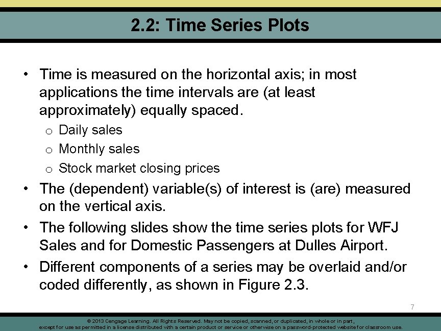
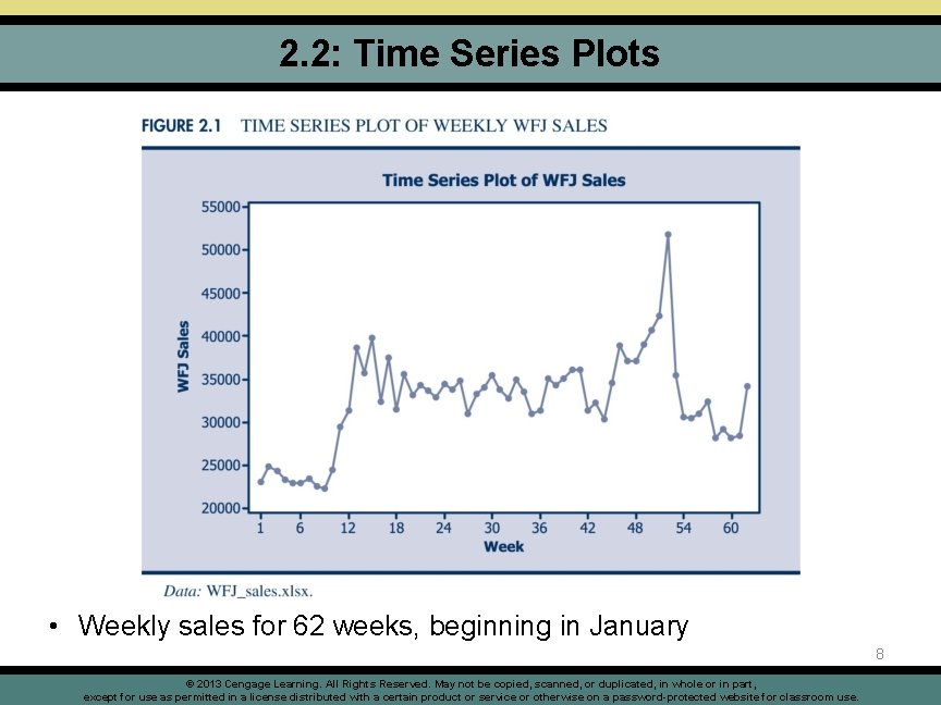
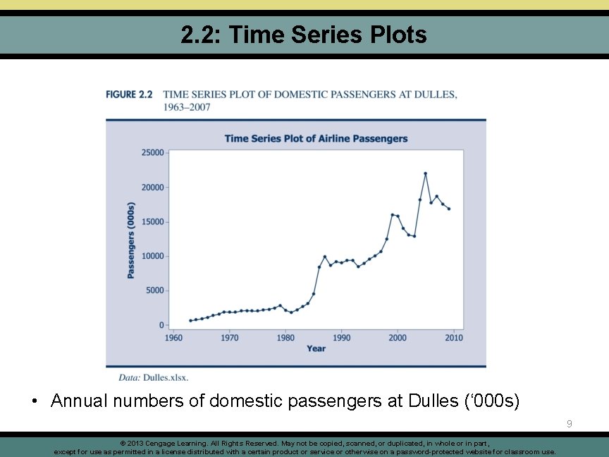
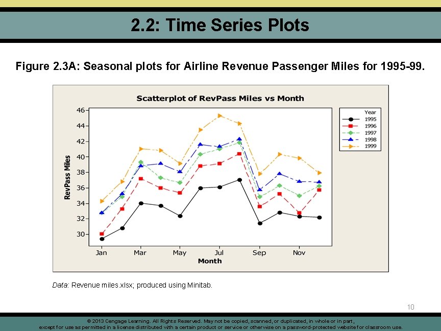
2. 2: Time Series Plots • Time is measured on the horizontal axis; in most applications the time intervals are (at least approximately) equally spaced. o Daily sales o Monthly sales o Stock market closing prices • The (dependent) variable(s) of interest is (are) measured on the vertical axis. • The following slides show the time series plots for WFJ Sales and for Domestic Passengers at Dulles Airport. • Different components of a series may be overlaid and/or coded differently, as shown in Figure 2. 3. 7 © 2013 Cengage Learning. All Rights Reserved. May not be copied, scanned, or duplicated, in whole or in part, except for use as permitted in a license distributed with a certain product or service or otherwise on a password-protected website for classroom use.

2. 2: Time Series Plots • Weekly sales for 62 weeks, beginning in January 8 © 2013 Cengage Learning. All Rights Reserved. May not be copied, scanned, or duplicated, in whole or in part, except for use as permitted in a license distributed with a certain product or service or otherwise on a password-protected website for classroom use.

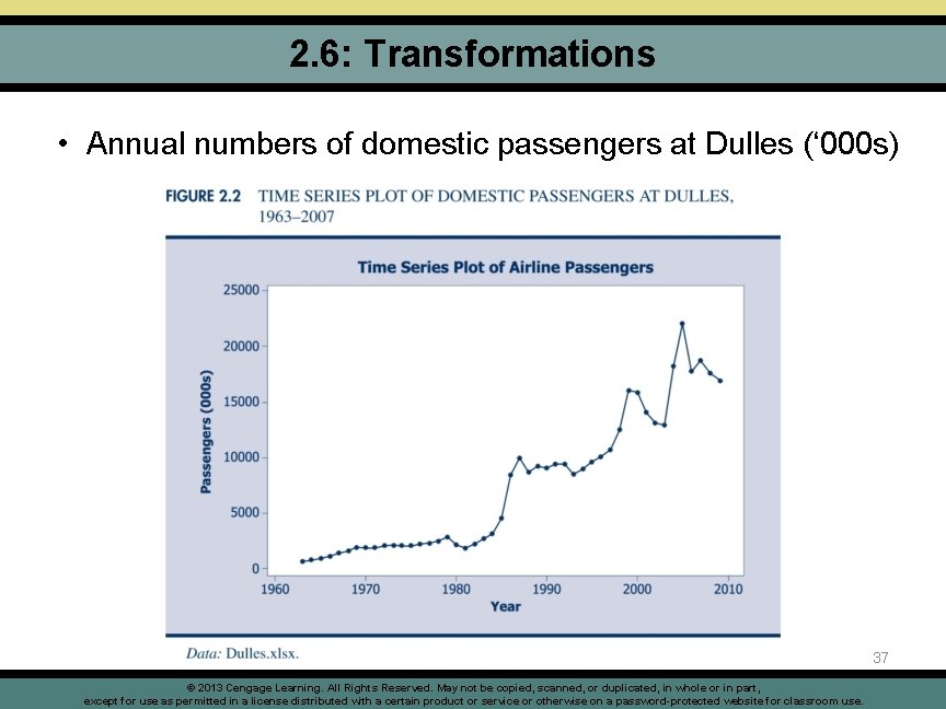
2. 2: Time Series Plots • Annual numbers of domestic passengers at Dulles (‘ 000 s) 9 © 2013 Cengage Learning. All Rights Reserved. May not be copied, scanned, or duplicated, in whole or in part, except for use as permitted in a license distributed with a certain product or service or otherwise on a password-protected website for classroom use.

2. 2: Time Series Plots Figure 2. 3 A: Seasonal plots for Airline Revenue Passenger Miles for 1995 -99. Data: Revenue miles. xlsx; produced using Minitab. 10 © 2013 Cengage Learning. All Rights Reserved. May not be copied, scanned, or duplicated, in whole or in part, except for use as permitted in a license distributed with a certain product or service or otherwise on a password-protected website for classroom use.

2. 2: Time Series Plots Figure 2. 3 B: Seasonal Plot across Years Data: Revenue miles. xlsx; produced using Minitab. 11 © 2013 Cengage Learning. All Rights Reserved. May not be copied, scanned, or duplicated, in whole or in part, except for use as permitted in a license distributed with a certain product or service or otherwise on a password-protected website for classroom use.

2. 2: Time Series Plots 12 © 2013 Cengage Learning. All Rights Reserved. May not be copied, scanned, or duplicated, in whole or in part, except for use as permitted in a license distributed with a certain product or service or otherwise on a password-protected website for classroom use.

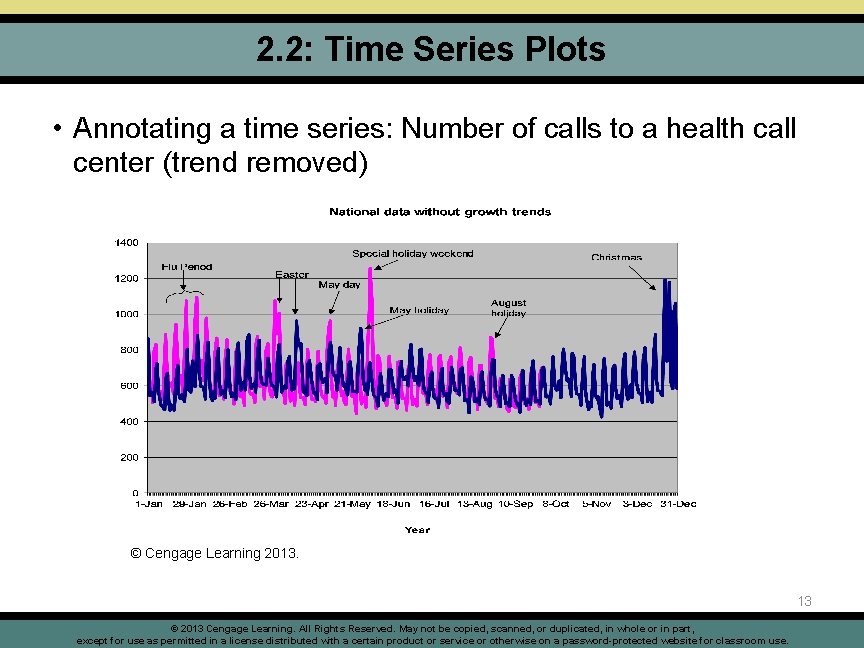
2. 2: Time Series Plots • Annotating a time series: Number of calls to a health call center (trend removed) © Cengage Learning 2013. 13 © 2013 Cengage Learning. All Rights Reserved. May not be copied, scanned, or duplicated, in whole or in part, except for use as permitted in a license distributed with a certain product or service or otherwise on a password-protected website for classroom use.

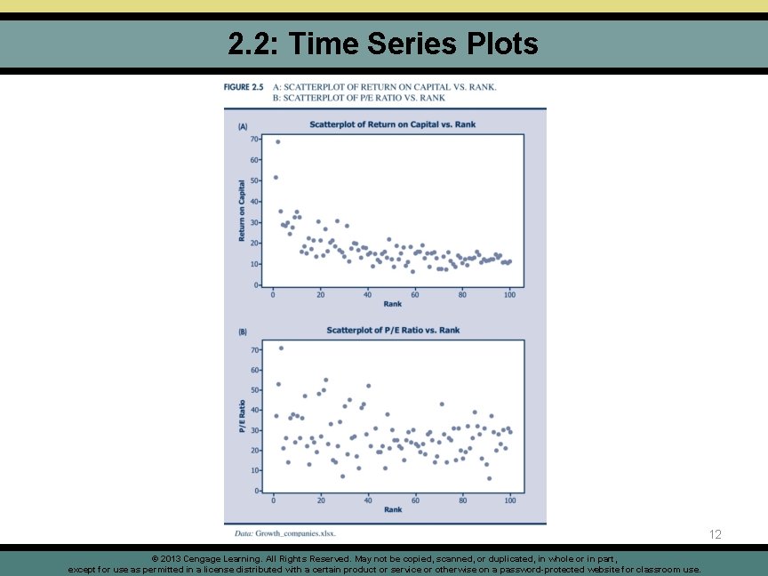
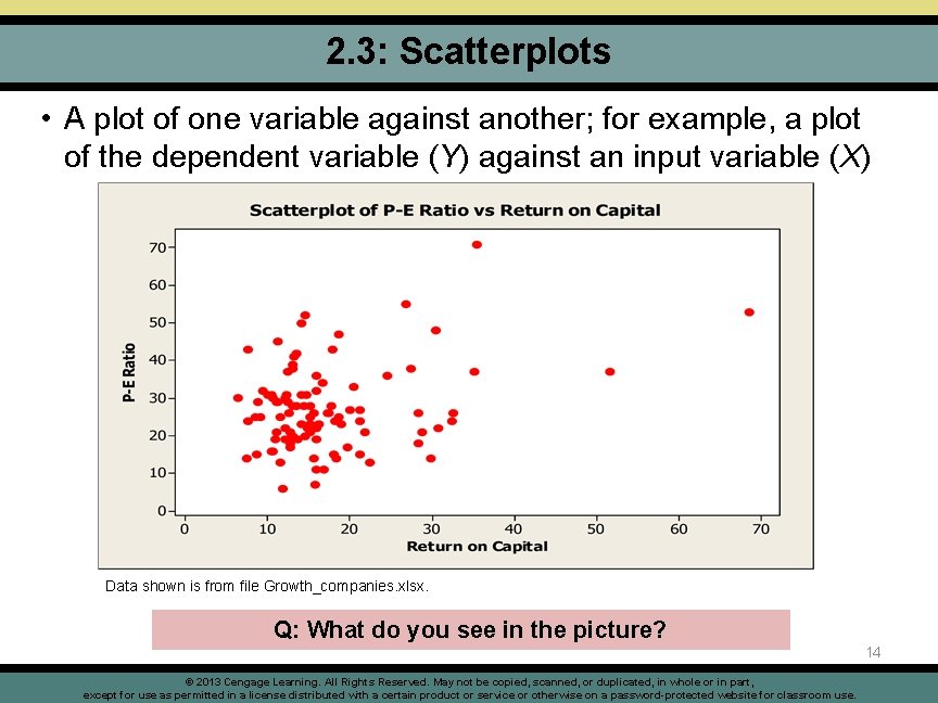
2. 3: Scatterplots • A plot of one variable against another; for example, a plot of the dependent variable (Y) against an input variable (X) Data shown is from file Growth_companies. xlsx. Q: What do you see in the picture? © 2013 Cengage Learning. All Rights Reserved. May not be copied, scanned, or duplicated, in whole or in part, except for use as permitted in a license distributed with a certain product or service or otherwise on a password-protected website for classroom use. 14

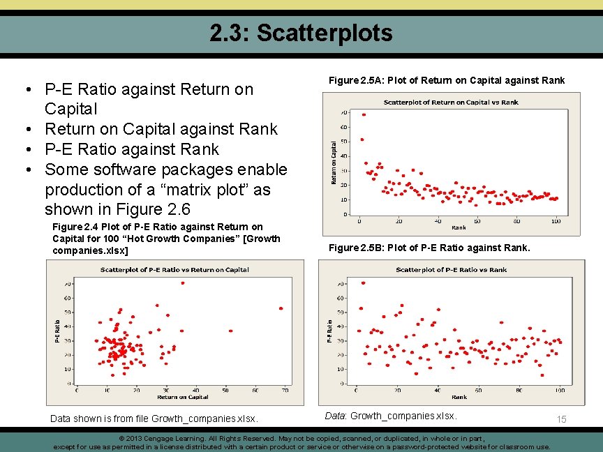
2. 3: Scatterplots • P-E Ratio against Return on Capital • Return on Capital against Rank • P-E Ratio against Rank • Some software packages enable production of a “matrix plot” as shown in Figure 2. 6 Figure 2. 4 Plot of P-E Ratio against Return on Capital for 100 “Hot Growth Companies” [Growth companies. xlsx] Data shown is from file Growth_companies. xlsx. Figure 2. 5 A: Plot of Return on Capital against Rank Figure 2. 5 B: Plot of P-E Ratio against Rank. Data: Growth_companies. xlsx. © 2013 Cengage Learning. All Rights Reserved. May not be copied, scanned, or duplicated, in whole or in part, except for use as permitted in a license distributed with a certain product or service or otherwise on a password-protected website for classroom use. 15

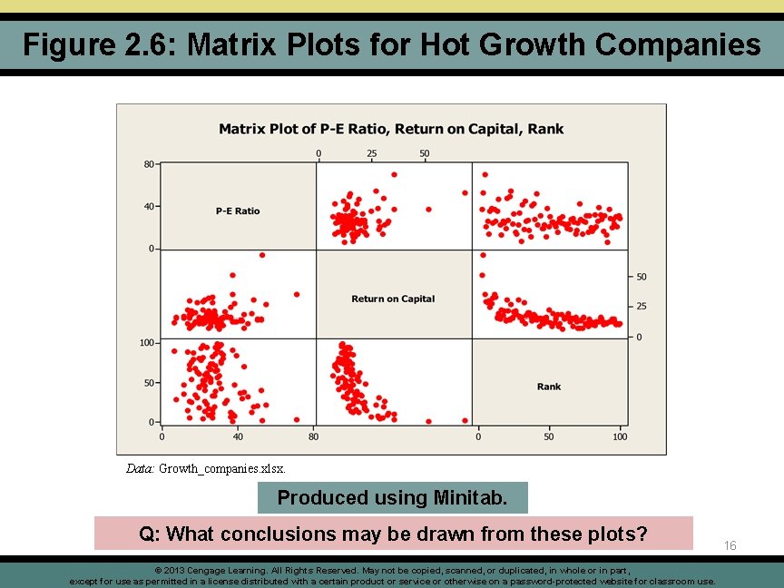
Figure 2. 6: Matrix Plots for Hot Growth Companies Data: Growth_companies. xlsx. Produced using Minitab. Q: What conclusions may be drawn from these plots? © 2013 Cengage Learning. All Rights Reserved. May not be copied, scanned, or duplicated, in whole or in part, except for use as permitted in a license distributed with a certain product or service or otherwise on a password-protected website for classroom use. 16

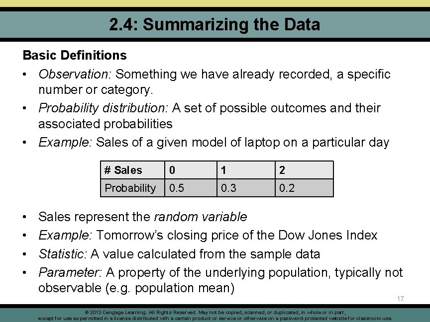
2. 4: Summarizing the Data Basic Definitions • Observation: Something we have already recorded, a specific number or category. • Probability distribution: A set of possible outcomes and their associated probabilities • Example: Sales of a given model of laptop on a particular day • • # Sales 0 1 2 Probability 0. 5 0. 3 0. 2 Sales represent the random variable Example: Tomorrow’s closing price of the Dow Jones Index Statistic: A value calculated from the sample data Parameter: A property of the underlying population, typically not observable (e. g. population mean) 17 © 2013 Cengage Learning. All Rights Reserved. May not be copied, scanned, or duplicated, in whole or in part, except for use as permitted in a license distributed with a certain product or service or otherwise on a password-protected website for classroom use.

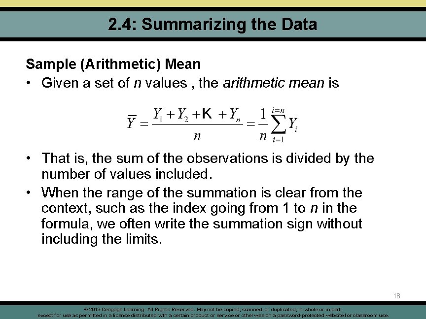
2. 4: Summarizing the Data Sample (Arithmetic) Mean • Given a set of n values , the arithmetic mean is • That is, the sum of the observations is divided by the number of values included. • When the range of the summation is clear from the context, such as the index going from 1 to n in the formula, we often write the summation sign without including the limits. 18 © 2013 Cengage Learning. All Rights Reserved. May not be copied, scanned, or duplicated, in whole or in part, except for use as permitted in a license distributed with a certain product or service or otherwise on a password-protected website for classroom use.

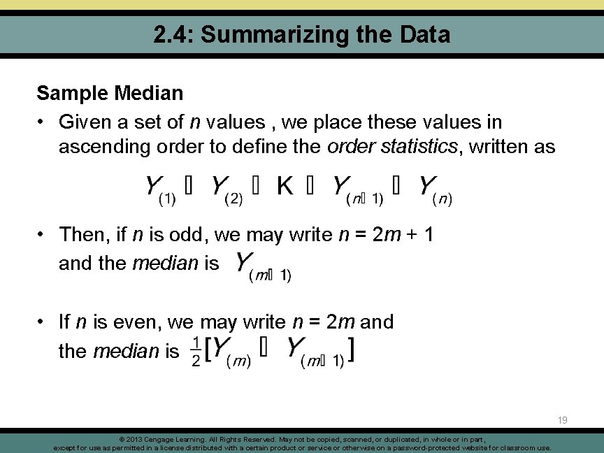
2. 4: Summarizing the Data Sample Median • Given a set of n values , we place these values in ascending order to define the order statistics, written as • Then, if n is odd, we may write n = 2 m + 1 and the median is • If n is even, we may write n = 2 m and the median is 19 © 2013 Cengage Learning. All Rights Reserved. May not be copied, scanned, or duplicated, in whole or in part, except for use as permitted in a license distributed with a certain product or service or otherwise on a password-protected website for classroom use.

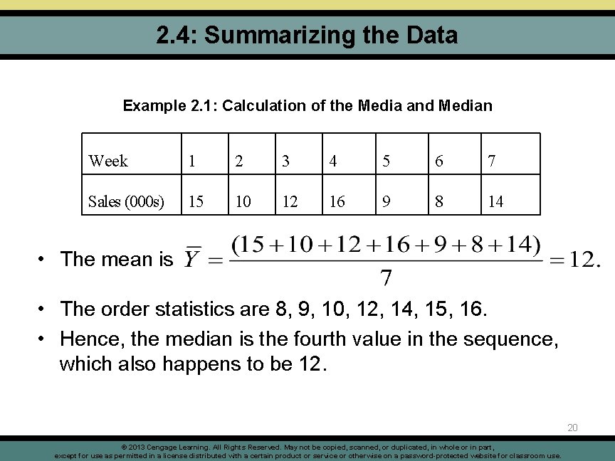
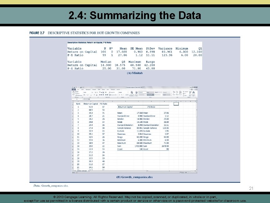
2. 4: Summarizing the Data Example 2. 1: Calculation of the Media and Median Week 1 2 3 4 5 6 7 Sales (000 s) 15 10 12 16 9 8 14 • The mean is • The order statistics are 8, 9, 10, 12, 14, 15, 16. • Hence, the median is the fourth value in the sequence, which also happens to be 12. 20 © 2013 Cengage Learning. All Rights Reserved. May not be copied, scanned, or duplicated, in whole or in part, except for use as permitted in a license distributed with a certain product or service or otherwise on a password-protected website for classroom use.

2. 4: Summarizing the Data 21 © 2013 Cengage Learning. All Rights Reserved. May not be copied, scanned, or duplicated, in whole or in part, except for use as permitted in a license distributed with a certain product or service or otherwise on a password-protected website for classroom use.

Discussion Question How would you describe house prices in an area if you were (a) planning to buy a home in the area (b) seeking to forecast revenues from the local property tax? Why? A. Median for both B. Mean for both C. Median for (a), mean for (b) D. Mean for (a), median for (b) 22 © 2013 Cengage Learning. All Rights Reserved. May not be copied, scanned, or duplicated, in whole or in part, except for use as permitted in a license distributed with a certain product or service or otherwise on a password-protected website for classroom use.

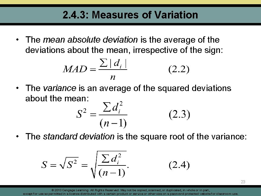
2. 4. 3: Measures of Variation • The mean absolute deviation is the average of the deviations about the mean, irrespective of the sign: • The variance is an average of the squared deviations about the mean: • The standard deviation is the square root of the variance: 23 © 2013 Cengage Learning. All Rights Reserved. May not be copied, scanned, or duplicated, in whole or in part, except for use as permitted in a license distributed with a certain product or service or otherwise on a password-protected website for classroom use.

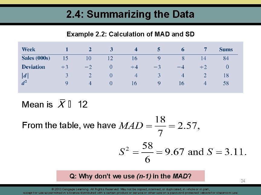
2. 4: Summarizing the Data Example 2. 2: Calculation of MAD and SD Mean is From the table, we have Q: Why don’t we use (n-1) in the MAD? © 2013 Cengage Learning. All Rights Reserved. May not be copied, scanned, or duplicated, in whole or in part, except for use as permitted in a license distributed with a certain product or service or otherwise on a password-protected website for classroom use. 24

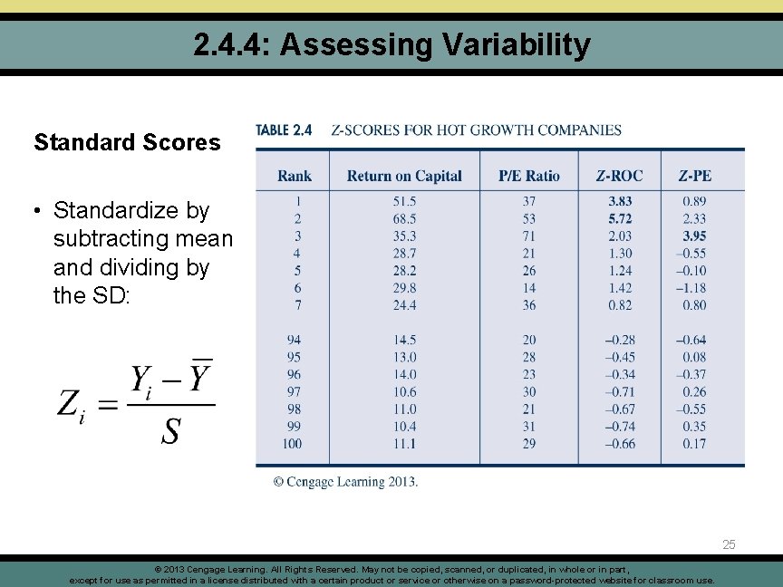
2. 4. 4: Assessing Variability Standard Scores • Standardize by subtracting mean and dividing by the SD: 25 © 2013 Cengage Learning. All Rights Reserved. May not be copied, scanned, or duplicated, in whole or in part, except for use as permitted in a license distributed with a certain product or service or otherwise on a password-protected website for classroom use.

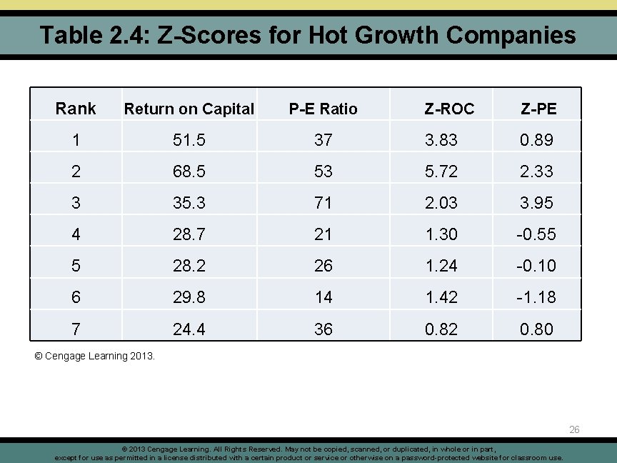
Table 2. 4: Z-Scores for Hot Growth Companies Rank Return on Capital P-E Ratio 1 51. 5 2 Z-ROC Z-PE 37 3. 83 0. 89 68. 5 53 5. 72 2. 33 3 35. 3 71 2. 03 3. 95 4 28. 7 21 1. 30 -0. 55 5 28. 2 26 1. 24 -0. 10 6 29. 8 14 1. 42 -1. 18 7 24. 4 36 0. 82 0. 80 © Cengage Learning 2013. 26 © 2013 Cengage Learning. All Rights Reserved. May not be copied, scanned, or duplicated, in whole or in part, except for use as permitted in a license distributed with a certain product or service or otherwise on a password-protected website for classroom use.

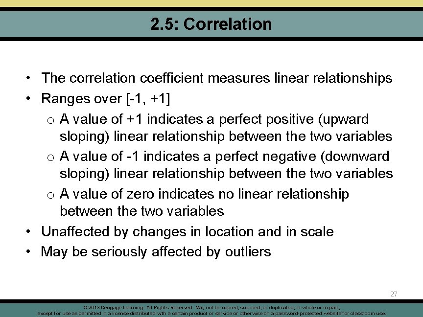
2. 5: Correlation • The correlation coefficient measures linear relationships • Ranges over [-1, +1] o A value of +1 indicates a perfect positive (upward sloping) linear relationship between the two variables o A value of -1 indicates a perfect negative (downward sloping) linear relationship between the two variables o A value of zero indicates no linear relationship between the two variables • Unaffected by changes in location and in scale • May be seriously affected by outliers 27 © 2013 Cengage Learning. All Rights Reserved. May not be copied, scanned, or duplicated, in whole or in part, except for use as permitted in a license distributed with a certain product or service or otherwise on a password-protected website for classroom use.

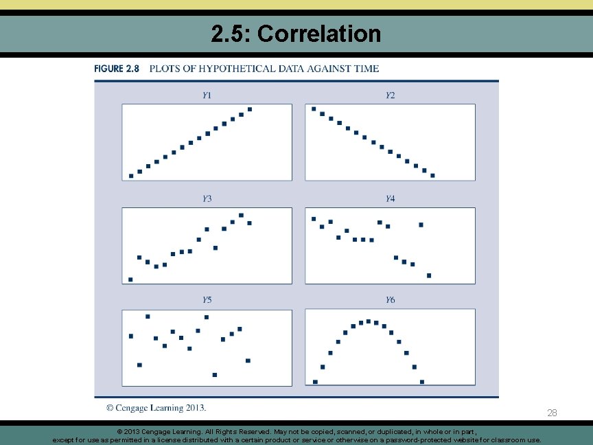
2. 5: Correlation 28 © 2013 Cengage Learning. All Rights Reserved. May not be copied, scanned, or duplicated, in whole or in part, except for use as permitted in a license distributed with a certain product or service or otherwise on a password-protected website for classroom use.

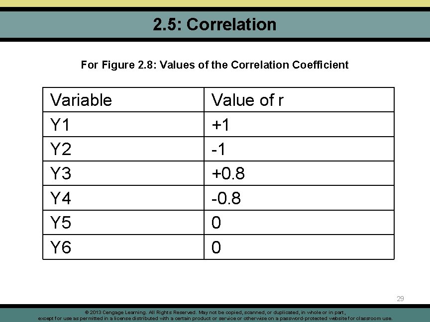
2. 5: Correlation For Figure 2. 8: Values of the Correlation Coefficient Variable Y 1 Y 2 Y 3 Y 4 Y 5 Y 6 Value of r +1 -1 +0. 8 -0. 8 0 0 29 © 2013 Cengage Learning. All Rights Reserved. May not be copied, scanned, or duplicated, in whole or in part, except for use as permitted in a license distributed with a certain product or service or otherwise on a password-protected website for classroom use.

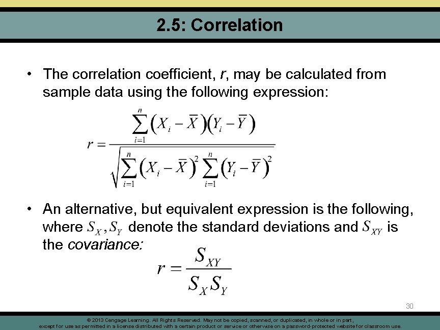
2. 5: Correlation • The correlation coefficient, r, may be calculated from sample data using the following expression: • An alternative, but equivalent expression is the following, where denote the standard deviations and is the covariance: 30 © 2013 Cengage Learning. All Rights Reserved. May not be copied, scanned, or duplicated, in whole or in part, except for use as permitted in a license distributed with a certain product or service or otherwise on a password-protected website for classroom use.

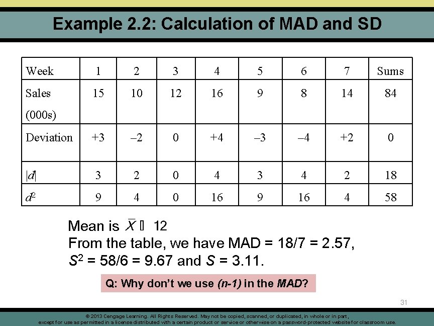
Example 2. 2: Calculation of MAD and SD Week 1 2 3 4 5 6 7 Sums Sales 15 10 12 16 9 8 14 84 Deviation +3 – 2 0 +4 – 3 – 4 +2 0 |d| 3 2 0 4 3 4 2 18 d 2 9 4 0 16 9 16 4 58 (000 s) Mean is From the table, we have MAD = 18/7 = 2. 57, S 2 = 58/6 = 9. 67 and S = 3. 11. Q: Why don’t we use (n-1) in the MAD? 31 © 2013 Cengage Learning. All Rights Reserved. May not be copied, scanned, or duplicated, in whole or in part, except for use as permitted in a license distributed with a certain product or service or otherwise on a password-protected website for classroom use.

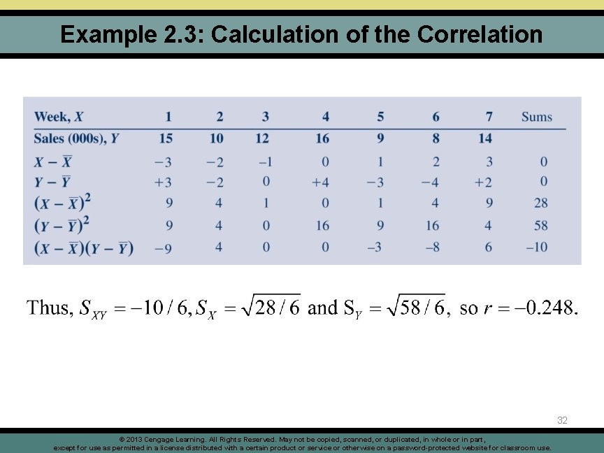
Example 2. 3: Calculation of the Correlation 32 © 2013 Cengage Learning. All Rights Reserved. May not be copied, scanned, or duplicated, in whole or in part, except for use as permitted in a license distributed with a certain product or service or otherwise on a password-protected website for classroom use.

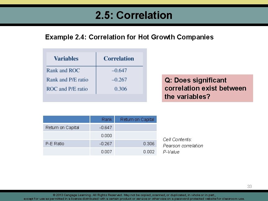
2. 5: Correlation Example 2. 4: Correlation for Hot Growth Companies Q: Does significant correlation exist between the variables? Rank Return on Capital -0. 647 0. 000 P-E Ratio -0. 267 0. 306 0. 007 0. 002 Cell Contents: Pearson correlation P-Value 33 © 2013 Cengage Learning. All Rights Reserved. May not be copied, scanned, or duplicated, in whole or in part, except for use as permitted in a license distributed with a certain product or service or otherwise on a password-protected website for classroom use.

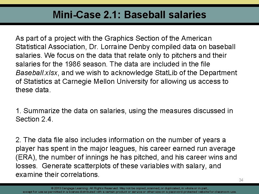
Mini-Case 2. 1: Baseball salaries As part of a project with the Graphics Section of the American Statistical Association, Dr. Lorraine Denby compiled data on baseball salaries. We focus on the data that relate only to pitchers and their salaries for the 1986 season. The data are included in the file Baseball. xlsx, and we wish to acknowledge Stat. Lib of the Department of Statistics at Carnegie Mellon University for allowing us access to these data. 1. Summarize the data on salaries, using the measures discussed in Section 2. 4. 2. The data file also includes information on the number of years a player has spent in the major leagues, his career earned run average (ERA), the number of innings he has pitched, and his career wins and losses. Generate scatterplots of these variables with salary, and examine their correlations. © 2013 Cengage Learning. All Rights Reserved. May not be copied, scanned, or duplicated, in whole or in part, except for use as permitted in a license distributed with a certain product or service or otherwise on a password-protected website for classroom use. 34

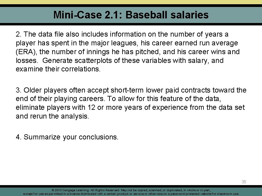
Mini-Case 2. 1: Baseball salaries 2. The data file also includes information on the number of years a player has spent in the major leagues, his career earned run average (ERA), the number of innings he has pitched, and his career wins and losses. Generate scatterplots of these variables with salary, and examine their correlations. 3. Older players often accept short-term lower paid contracts toward the end of their playing careers. To allow for this feature of the data, eliminate players with 12 or more years of experience from the data set and rerun the analysis. 4. Summarize your conclusions. 35 © 2013 Cengage Learning. All Rights Reserved. May not be copied, scanned, or duplicated, in whole or in part, except for use as permitted in a license distributed with a certain product or service or otherwise on a password-protected website for classroom use.

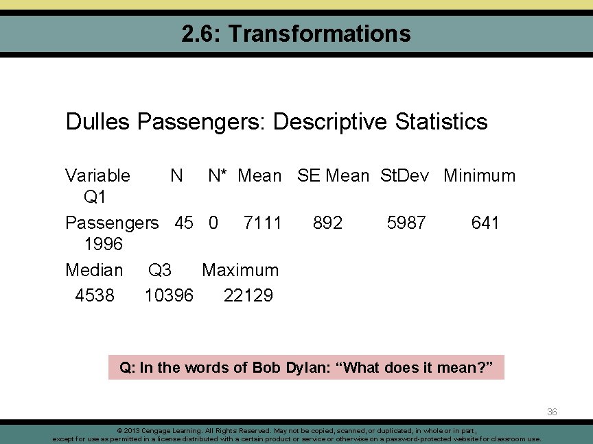
2. 6: Transformations Dulles Passengers: Descriptive Statistics Variable N N* Mean SE Mean St. Dev Minimum Q 1 Passengers 45 0 7111 892 5987 641 1996 Median Q 3 Maximum 4538 10396 22129 Q: In the words of Bob Dylan: “What does it mean? ” 36 © 2013 Cengage Learning. All Rights Reserved. May not be copied, scanned, or duplicated, in whole or in part, except for use as permitted in a license distributed with a certain product or service or otherwise on a password-protected website for classroom use.

2. 6: Transformations • Annual numbers of domestic passengers at Dulles (‘ 000 s) 37 © 2013 Cengage Learning. All Rights Reserved. May not be copied, scanned, or duplicated, in whole or in part, except for use as permitted in a license distributed with a certain product or service or otherwise on a password-protected website for classroom use.

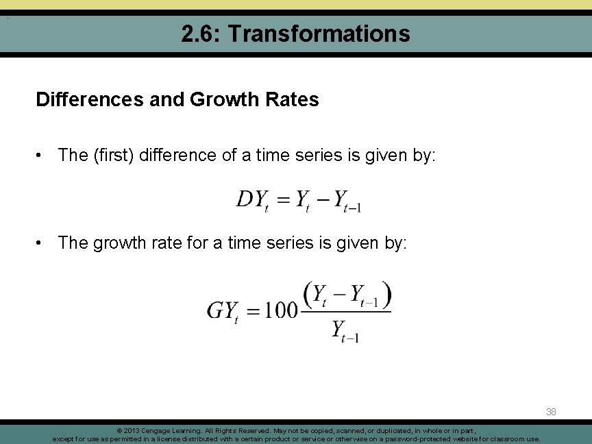
. 2. 6: Transformations Differences and Growth Rates • The (first) difference of a time series is given by: • The growth rate for a time series is given by: 38 © 2013 Cengage Learning. All Rights Reserved. May not be copied, scanned, or duplicated, in whole or in part, except for use as permitted in a license distributed with a certain product or service or otherwise on a password-protected website for classroom use.

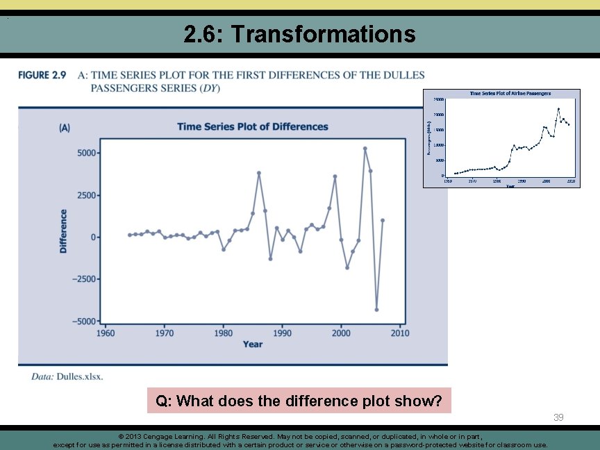
. 2. 6: Transformations Q: What does the difference plot show? 39 © 2013 Cengage Learning. All Rights Reserved. May not be copied, scanned, or duplicated, in whole or in part, except for use as permitted in a license distributed with a certain product or service or otherwise on a password-protected website for classroom use.

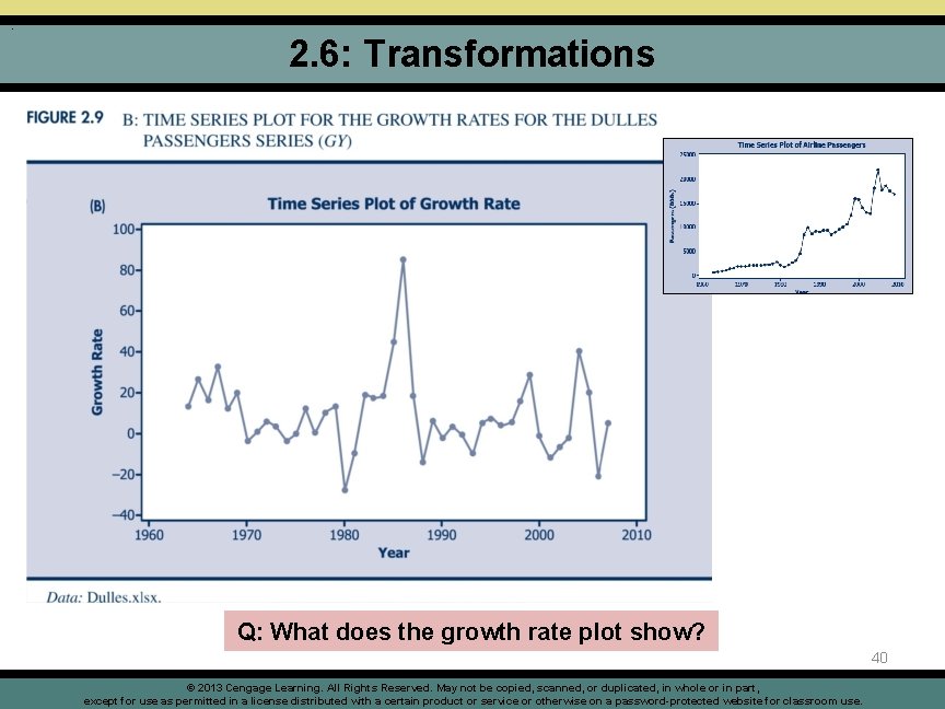
. 2. 6: Transformations Q: What does the growth rate plot show? 40 © 2013 Cengage Learning. All Rights Reserved. May not be copied, scanned, or duplicated, in whole or in part, except for use as permitted in a license distributed with a certain product or service or otherwise on a password-protected website for classroom use.

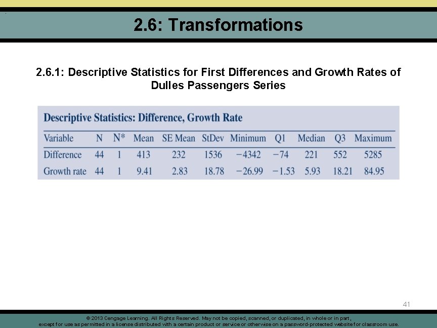
. 2. 6: Transformations 2. 6. 1: Descriptive Statistics for First Differences and Growth Rates of Dulles Passengers Series 41 © 2013 Cengage Learning. All Rights Reserved. May not be copied, scanned, or duplicated, in whole or in part, except for use as permitted in a license distributed with a certain product or service or otherwise on a password-protected website for classroom use.

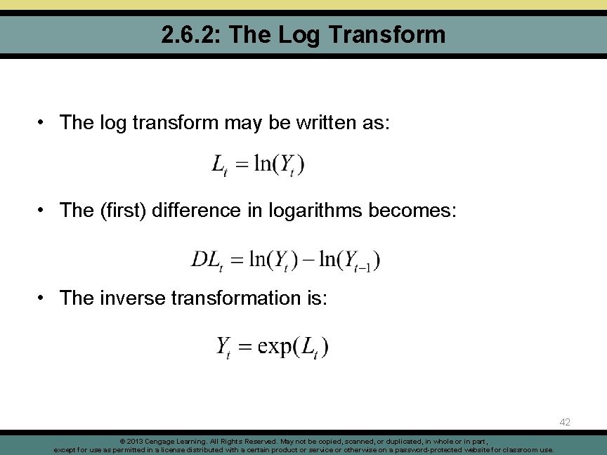
2. 6. 2: The Log Transform • The log transform may be written as: • The (first) difference in logarithms becomes: • The inverse transformation is: 42 © 2013 Cengage Learning. All Rights Reserved. May not be copied, scanned, or duplicated, in whole or in part, except for use as permitted in a license distributed with a certain product or service or otherwise on a password-protected website for classroom use.

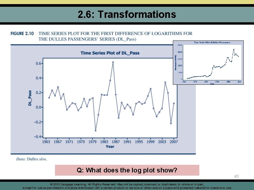
2. 6: Transformations Q: What does the log plot show? © 2013 Cengage Learning. All Rights Reserved. May not be copied, scanned, or duplicated, in whole or in part, except for use as permitted in a license distributed with a certain product or service or otherwise on a password-protected website for classroom use. 43

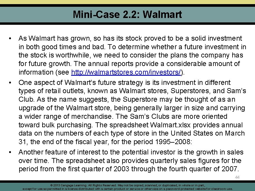
Mini-Case 2. 2: Walmart • As Walmart has grown, so has its stock proved to be a solid investment in both good times and bad. To determine whether a future investment in the stock is worthwhile, we need to consider the plans the company has for future growth. The annual reports provide a considerable amount of information (see http: //walmartstores. com/investors/). • One aspect of Walmart’s future strategy is its investment in different types of retail outlets, known as Walmart stores, Superstores, and Sam’s Club. As the name suggests, the Superstore may be thought of as an upgrade of the Walmart store, being generally larger in size and carrying a wider range of merchandise. The Sam’s Clubs are more oriented toward bulk purchasing. The spreadsheet Walmart. xlsx provides annual data on the numbers of each type of store in the United States on March 31, the end of the fiscal year, for the period 1995– 2008: • Another feature of interest to the potential investor is the growth in sales over time. The spreadsheet also provides quarterly sales figures for the period from the first quarter of 2003 through the fourth quarter of 2007. 44 © 2013 Cengage Learning. All Rights Reserved. May not be copied, scanned, or duplicated, in whole or in part, except for use as permitted in a license distributed with a certain product or service or otherwise on a password-protected website for classroom use.

Mini-Case 2. 3: Length of Recessions The data in recessions. xlsx summarize the length of each recession in the period 1929 - 2008, as determined by the National Bureau of Economic Research. 1. 2. 3. 4. Calculate the average length of a recession and provide a 95 percent confidence interval for this quantity. Interpret the result. Calculate the average time between recessions and provide a 95 percent confidence interval for this quantity. Interpret the result. Is there any correlation between the length of a recession and the period of growth immediately preceding it referred to as ‘Gap’ in the table? Is there any correlation between the length of a recession and the period of growth immediately following a recession? 45 © 2013 Cengage Learning. All Rights Reserved. May not be copied, scanned, or duplicated, in whole or in part, except for use as permitted in a license distributed with a certain product or service or otherwise on a password-protected website for classroom use.

2. 7: How to Measure Forecasting Accuracy • • • What do you need from the forecasting activity? Quantitative Accuracy Timing Accuracy How do we measure these? Asymmetric measures? o “The thrill of winning is much less than the agony of defeat. ” Michigan State Football Coach [paraphrased] 46 © 2013 Cengage Learning. All Rights Reserved. May not be copied, scanned, or duplicated, in whole or in part, except for use as permitted in a license distributed with a certain product or service or otherwise on a password-protected website for classroom use.

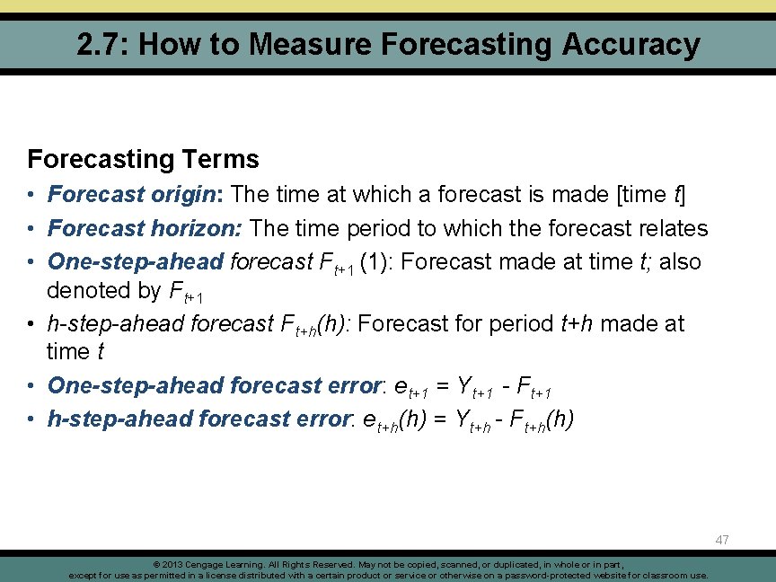
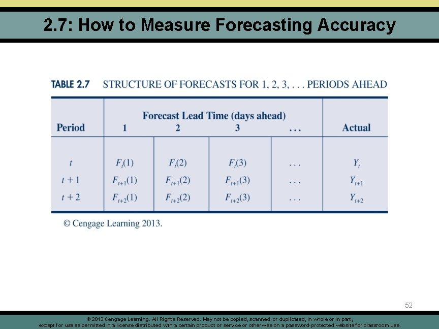
2. 7: How to Measure Forecasting Accuracy Forecasting Terms • Forecast origin: The time at which a forecast is made [time t] • Forecast horizon: The time period to which the forecast relates • One-step-ahead forecast Ft+1 (1): Forecast made at time t; also denoted by Ft+1 • h-step-ahead forecast Ft+h(h): Forecast for period t+h made at time t • One-step-ahead forecast error: et+1 = Yt+1 - Ft+1 • h-step-ahead forecast error: et+h(h) = Yt+h - Ft+h(h) 47 © 2013 Cengage Learning. All Rights Reserved. May not be copied, scanned, or duplicated, in whole or in part, except for use as permitted in a license distributed with a certain product or service or otherwise on a password-protected website for classroom use.

2. 7: How to Measure Forecasting Accuracy 48 © 2013 Cengage Learning. All Rights Reserved. May not be copied, scanned, or duplicated, in whole or in part, except for use as permitted in a license distributed with a certain product or service or otherwise on a password-protected website for classroom use.

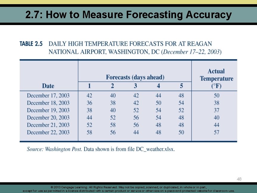
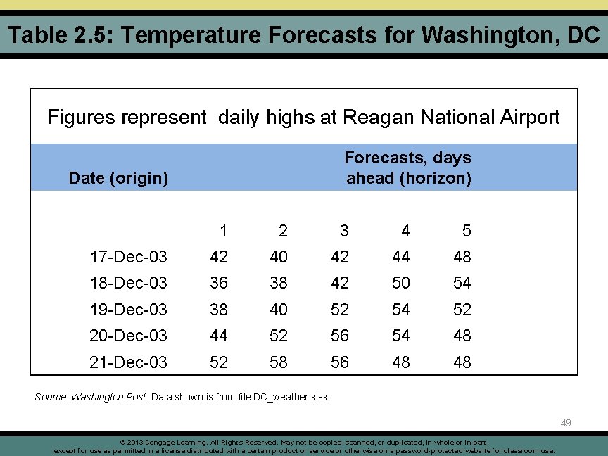
Table 2. 5: Temperature Forecasts for Washington, DC Figures represent daily highs at Reagan National Airport Forecasts, days ahead (horizon) Date (origin) 1 2 3 4 5 17 -Dec-03 42 40 42 44 48 18 -Dec-03 36 38 42 50 54 19 -Dec-03 38 40 52 54 52 20 -Dec-03 44 52 56 54 48 21 -Dec-03 52 58 56 48 48 Source: Washington Post. Data shown is from file DC_weather. xlsx. 49 © 2013 Cengage Learning. All Rights Reserved. May not be copied, scanned, or duplicated, in whole or in part, except for use as permitted in a license distributed with a certain product or service or otherwise on a password-protected website for classroom use.

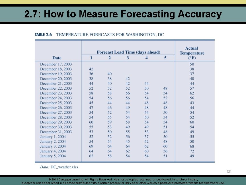
2. 7: How to Measure Forecasting Accuracy 50 © 2013 Cengage Learning. All Rights Reserved. May not be copied, scanned, or duplicated, in whole or in part, except for use as permitted in a license distributed with a certain product or service or otherwise on a password-protected website for classroom use.

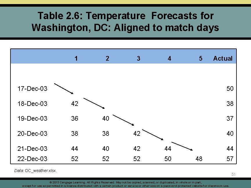
Table 2. 6: Temperature Forecasts for Washington, DC: Aligned to match days 1 2 3 4 5 17 -Dec-03 Actual 50 18 -Dec-03 42 38 19 -Dec-03 36 40 20 -Dec-03 38 38 42 21 -Dec-03 44 40 42 44 22 -Dec-03 52 52 52 50 37 40 44 48 57 Data: DC_weather. xlsx. © 2013 Cengage Learning. All Rights Reserved. May not be copied, scanned, or duplicated, in whole or in part, except for use as permitted in a license distributed with a certain product or service or otherwise on a password-protected website for classroom use. 51

2. 7: How to Measure Forecasting Accuracy 52 © 2013 Cengage Learning. All Rights Reserved. May not be copied, scanned, or duplicated, in whole or in part, except for use as permitted in a license distributed with a certain product or service or otherwise on a password-protected website for classroom use.

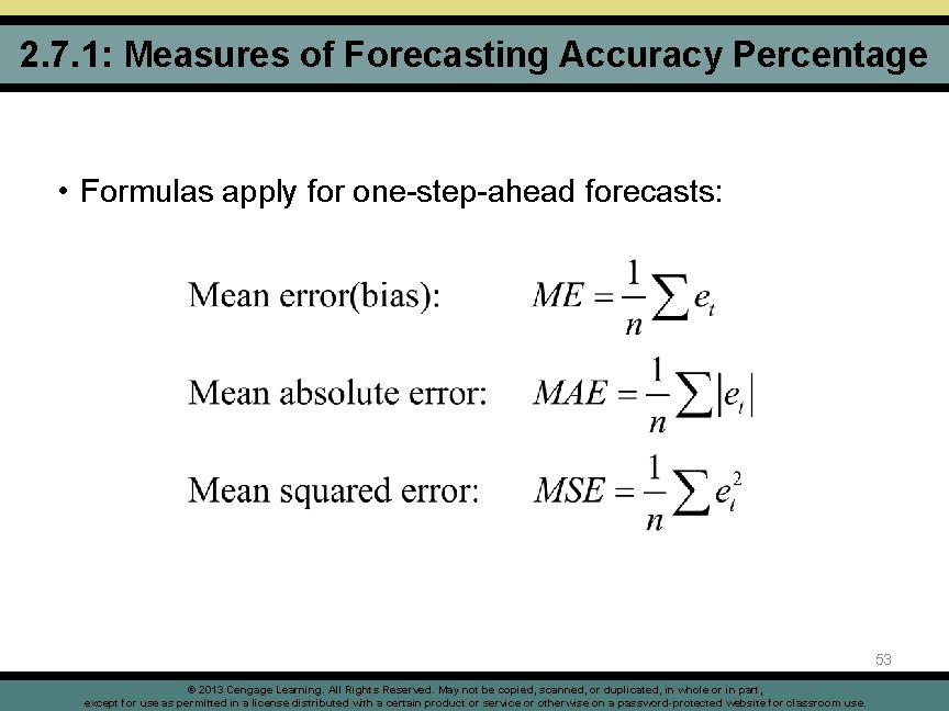
2. 7. 1: Measures of Forecasting Accuracy Percentage • Formulas apply for one-step-ahead forecasts: 53 © 2013 Cengage Learning. All Rights Reserved. May not be copied, scanned, or duplicated, in whole or in part, except for use as permitted in a license distributed with a certain product or service or otherwise on a password-protected website for classroom use.

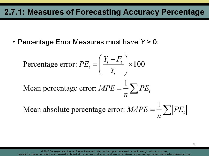
2. 7. 1: Measures of Forecasting Accuracy Percentage • Percentage Error Measures must have Y > 0: 54 © 2013 Cengage Learning. All Rights Reserved. May not be copied, scanned, or duplicated, in whole or in part, except for use as permitted in a license distributed with a certain product or service or otherwise on a password-protected website for classroom use.

2. 7. 2: Measures of Absolute Error Mean Absolute Scaled Error [MASE] 55 © 2013 Cengage Learning. All Rights Reserved. May not be copied, scanned, or duplicated, in whole or in part, except for use as permitted in a license distributed with a certain product or service or otherwise on a password-protected website for classroom use.

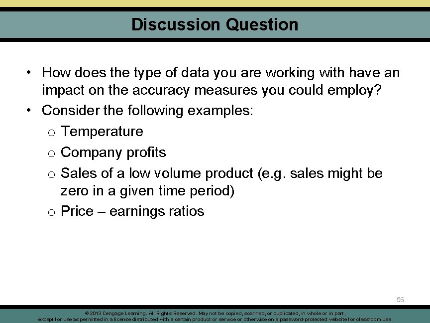
Discussion Question • How does the type of data you are working with have an impact on the accuracy measures you could employ? • Consider the following examples: o Temperature o Company profits o Sales of a low volume product (e. g. sales might be zero in a given time period) o Price – earnings ratios 56 © 2013 Cengage Learning. All Rights Reserved. May not be copied, scanned, or duplicated, in whole or in part, except for use as permitted in a license distributed with a certain product or service or otherwise on a password-protected website for classroom use.

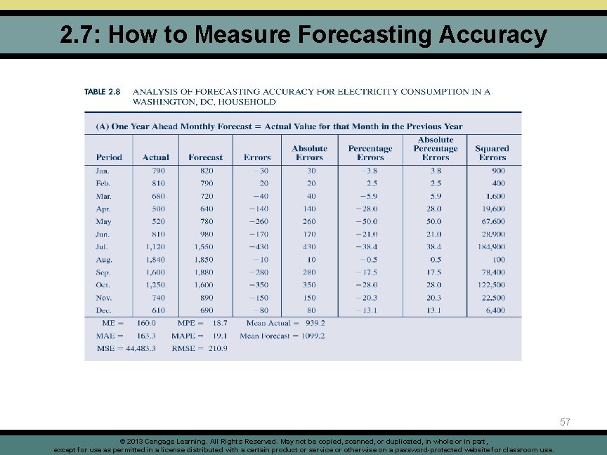
2. 7: How to Measure Forecasting Accuracy 57 © 2013 Cengage Learning. All Rights Reserved. May not be copied, scanned, or duplicated, in whole or in part, except for use as permitted in a license distributed with a certain product or service or otherwise on a password-protected website for classroom use.

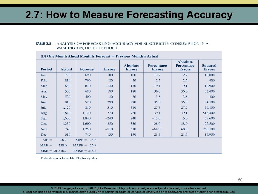
2. 7: How to Measure Forecasting Accuracy 58 © 2013 Cengage Learning. All Rights Reserved. May not be copied, scanned, or duplicated, in whole or in part, except for use as permitted in a license distributed with a certain product or service or otherwise on a password-protected website for classroom use.

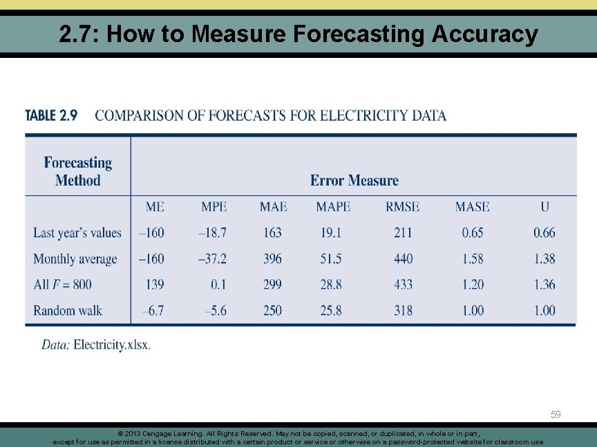
2. 7: How to Measure Forecasting Accuracy 59 © 2013 Cengage Learning. All Rights Reserved. May not be copied, scanned, or duplicated, in whole or in part, except for use as permitted in a license distributed with a certain product or service or otherwise on a password-protected website for classroom use.

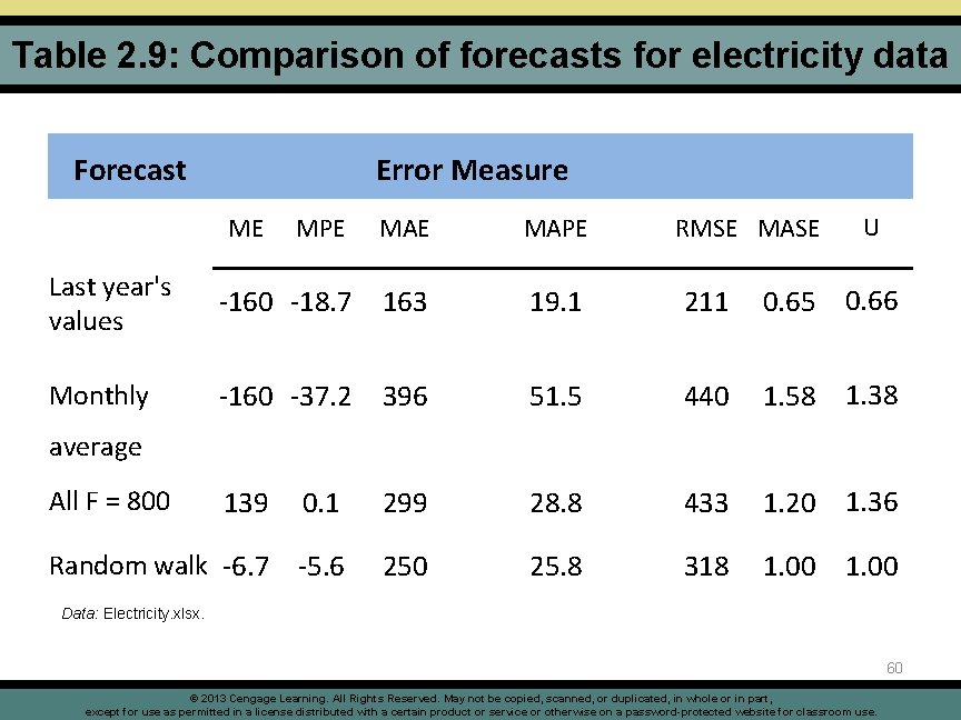
Table 2. 9: Comparison of forecasts for electricity data Forecast Error Measure ME MPE RMSE MASE U MAE MAPE Last year's values -160 -18. 7 163 19. 1 211 0. 65 0. 66 Monthly -160 -37. 2 396 51. 5 440 1. 58 1. 38 139 average 0. 1 299 28. 8 433 1. 20 1. 36 Random walk -6. 7 -5. 6 250 25. 8 318 1. 00 All F = 800 Data: Electricity. xlsx. 60 © 2013 Cengage Learning. All Rights Reserved. May not be copied, scanned, or duplicated, in whole or in part, except for use as permitted in a license distributed with a certain product or service or otherwise on a password-protected website for classroom use.

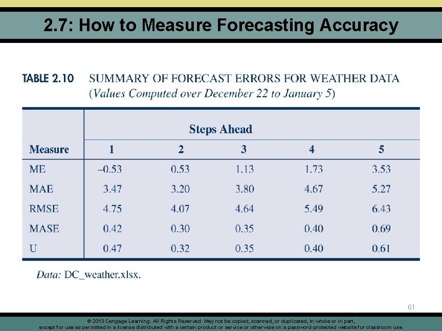
2. 7: How to Measure Forecasting Accuracy 61 © 2013 Cengage Learning. All Rights Reserved. May not be copied, scanned, or duplicated, in whole or in part, except for use as permitted in a license distributed with a certain product or service or otherwise on a password-protected website for classroom use.

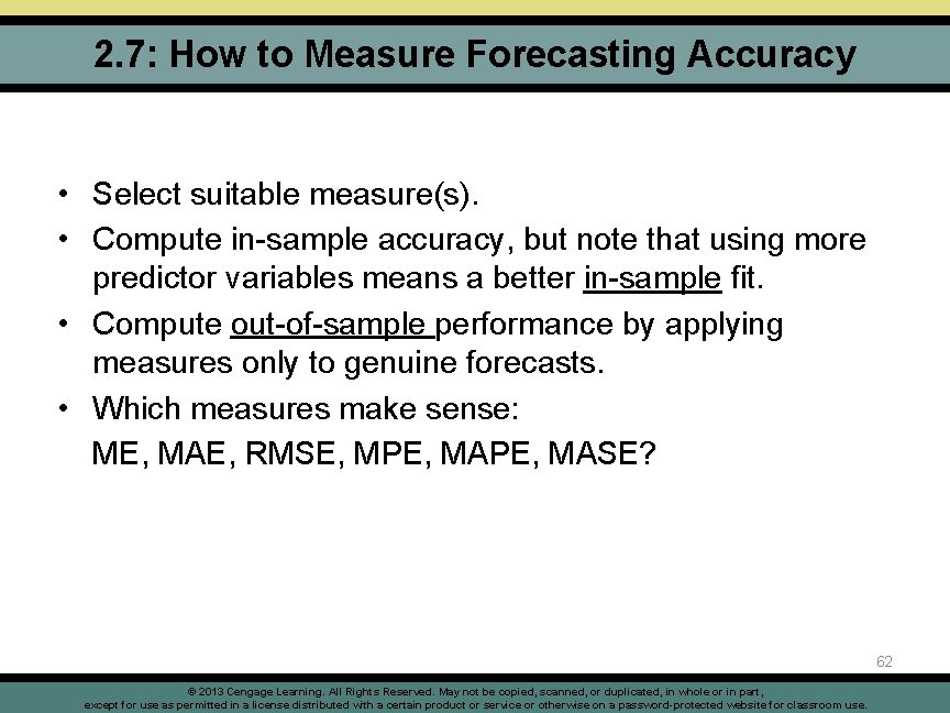
2. 7: How to Measure Forecasting Accuracy • Select suitable measure(s). • Compute in-sample accuracy, but note that using more predictor variables means a better in-sample fit. • Compute out-of-sample performance by applying measures only to genuine forecasts. • Which measures make sense: ME, MAE, RMSE, MPE, MASE? 62 © 2013 Cengage Learning. All Rights Reserved. May not be copied, scanned, or duplicated, in whole or in part, except for use as permitted in a license distributed with a certain product or service or otherwise on a password-protected website for classroom use.

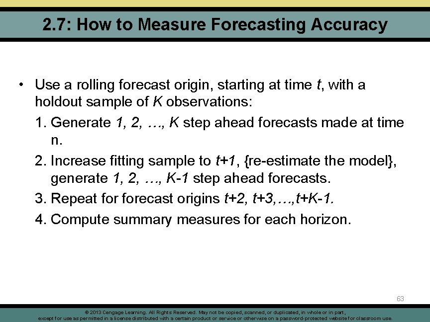
2. 7: How to Measure Forecasting Accuracy • Use a rolling forecast origin, starting at time t, with a holdout sample of K observations: 1. Generate 1, 2, …, K step ahead forecasts made at time n. 2. Increase fitting sample to t+1, {re-estimate the model}, generate 1, 2, …, K-1 step ahead forecasts. 3. Repeat forecast origins t+2, t+3, …, t+K-1. 4. Compute summary measures for each horizon. 63 © 2013 Cengage Learning. All Rights Reserved. May not be copied, scanned, or duplicated, in whole or in part, except for use as permitted in a license distributed with a certain product or service or otherwise on a password-protected website for classroom use.

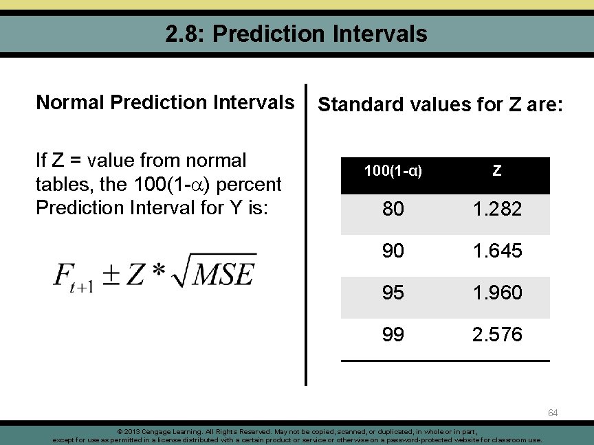
2. 8: Prediction Intervals Normal Prediction Intervals If Z = value from normal tables, the 100(1 - ) percent Prediction Interval for Y is: Standard values for Z are: 100(1 -α) Z 80 1. 282 90 1. 645 95 1. 960 99 2. 576 64 © 2013 Cengage Learning. All Rights Reserved. May not be copied, scanned, or duplicated, in whole or in part, except for use as permitted in a license distributed with a certain product or service or otherwise on a password-protected website for classroom use.

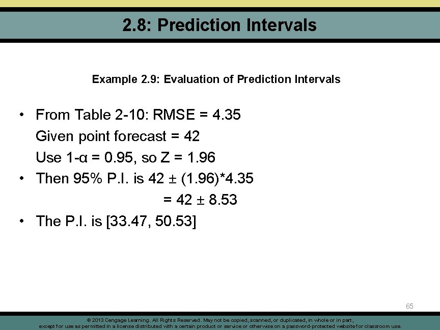
2. 8: Prediction Intervals Example 2. 9: Evaluation of Prediction Intervals • From Table 2 -10: RMSE = 4. 35 Given point forecast = 42 Use 1 -α = 0. 95, so Z = 1. 96 • Then 95% P. I. is 42 ± (1. 96)*4. 35 = 42 ± 8. 53 • The P. I. is [33. 47, 50. 53] 65 © 2013 Cengage Learning. All Rights Reserved. May not be copied, scanned, or duplicated, in whole or in part, except for use as permitted in a license distributed with a certain product or service or otherwise on a password-protected website for classroom use.

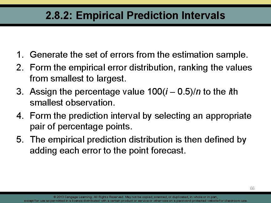
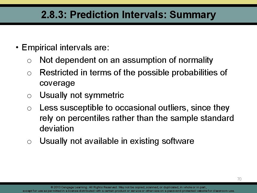
2. 8. 2: Empirical Prediction Intervals 1. Generate the set of errors from the estimation sample. 2. Form the empirical error distribution, ranking the values from smallest to largest. 3. Assign the percentage value 100(i – 0. 5)/n to the ith smallest observation. 4. Form the prediction interval by selecting an appropriate pair of percentage points. 5. The empirical prediction distribution is then defined by adding each error to the point forecast. 66 © 2013 Cengage Learning. All Rights Reserved. May not be copied, scanned, or duplicated, in whole or in part, except for use as permitted in a license distributed with a certain product or service or otherwise on a password-protected website for classroom use.

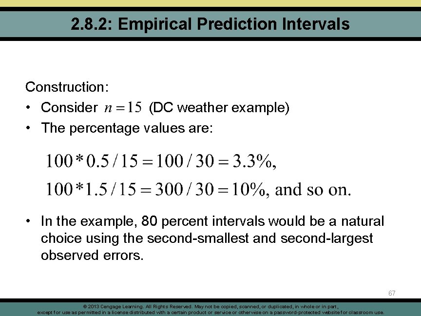
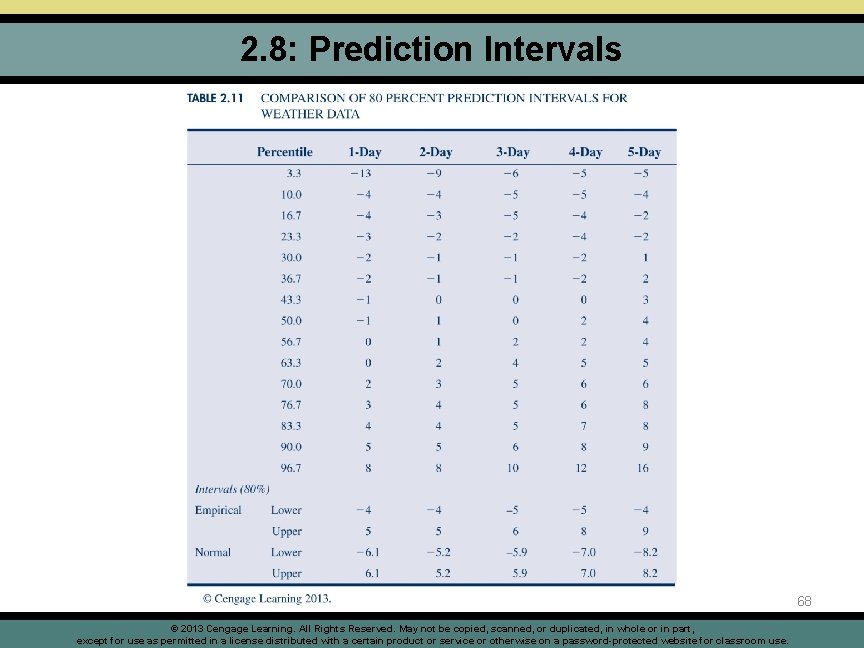
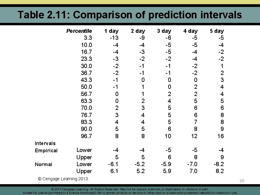
2. 8. 2: Empirical Prediction Intervals Construction: • Consider (DC weather example) • The percentage values are: • In the example, 80 percent intervals would be a natural choice using the second-smallest and second-largest observed errors. 67 © 2013 Cengage Learning. All Rights Reserved. May not be copied, scanned, or duplicated, in whole or in part, except for use as permitted in a license distributed with a certain product or service or otherwise on a password-protected website for classroom use.

2. 8: Prediction Intervals 68 © 2013 Cengage Learning. All Rights Reserved. May not be copied, scanned, or duplicated, in whole or in part, except for use as permitted in a license distributed with a certain product or service or otherwise on a password-protected website for classroom use.

Table 2. 11: Comparison of prediction intervals Intervals Empirical Normal Percentile 1 day 2 day 3 day 4 day 5 day 3. 3 10. 0 16. 7 23. 3 30. 0 36. 7 43. 3 50. 0 56. 7 63. 3 70. 0 76. 7 83. 3 90. 0 96. 7 -13 -4 -4 -3 -2 -2 -1 -1 0 0 2 3 4 5 8 -9 -4 -3 -2 -1 -1 0 1 1 2 3 4 4 5 8 -6 -5 -5 -2 -1 -1 0 0 2 4 5 5 5 6 10 -5 -5 -4 -4 -2 -2 0 2 2 5 6 6 7 8 12 -5 -4 -2 -2 1 2 3 4 4 5 6 8 8 9 16 Lower Upper -4 5 -6. 1 -4 5 -5. 2 -5 6 -5. 9 -5 8 -7. 0 -4 9 -8. 2 © Cengage Learning 2013. © 2013 Cengage Learning. All Rights Reserved. May not be copied, scanned, or duplicated, in whole or in part, except for use as permitted in a license distributed with a certain product or service or otherwise on a password-protected website for classroom use. 69

2. 8. 3: Prediction Intervals: Summary • Empirical intervals are: o Not dependent on an assumption of normality o Restricted in terms of the possible probabilities of coverage o Usually not symmetric o Less susceptible to occasional outliers, since they rely on percentiles rather than the sample standard deviation o Usually not available in existing software 70 © 2013 Cengage Learning. All Rights Reserved. May not be copied, scanned, or duplicated, in whole or in part, except for use as permitted in a license distributed with a certain product or service or otherwise on a password-protected website for classroom use.

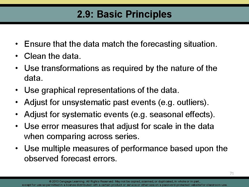
2. 9: Basic Principles • Ensure that the data match the forecasting situation. • Clean the data. • Use transformations as required by the nature of the data. • Use graphical representations of the data. • Adjust for unsystematic past events (e. g. outliers). • Adjust for systematic events (e. g. seasonal effects). • Use error measures that adjust for scale in the data when comparing across series. • Use multiple measures of performance based upon the observed forecast errors. 71 © 2013 Cengage Learning. All Rights Reserved. May not be copied, scanned, or duplicated, in whole or in part, except for use as permitted in a license distributed with a certain product or service or otherwise on a password-protected website for classroom use.

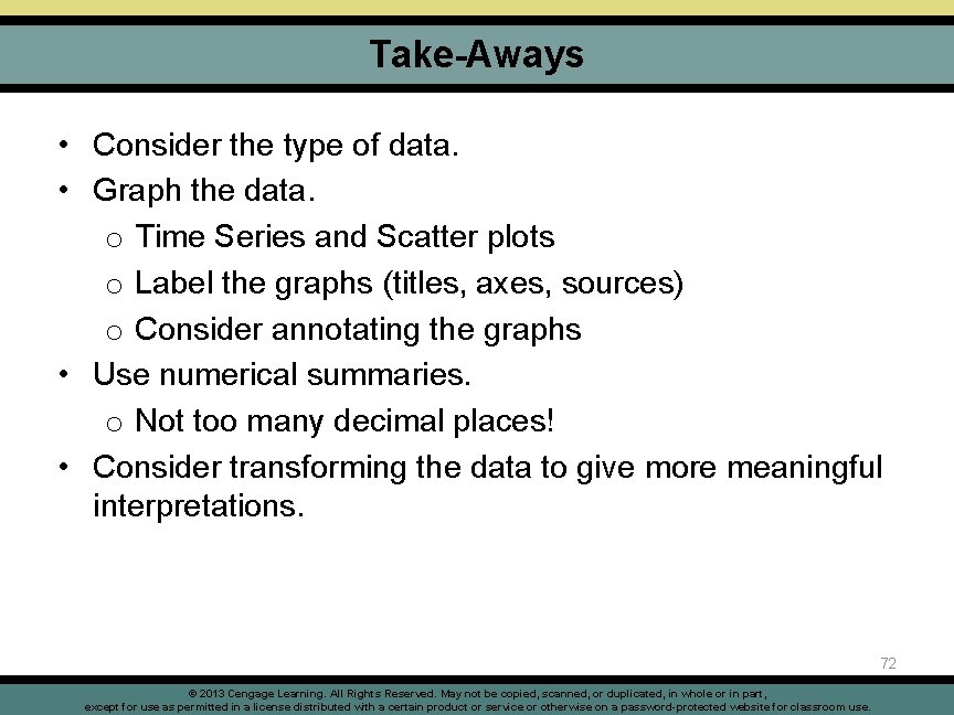
Take-Aways • Consider the type of data. • Graph the data. o Time Series and Scatter plots o Label the graphs (titles, axes, sources) o Consider annotating the graphs • Use numerical summaries. o Not too many decimal places! • Consider transforming the data to give more meaningful interpretations. 72 © 2013 Cengage Learning. All Rights Reserved. May not be copied, scanned, or duplicated, in whole or in part, except for use as permitted in a license distributed with a certain product or service or otherwise on a password-protected website for classroom use.

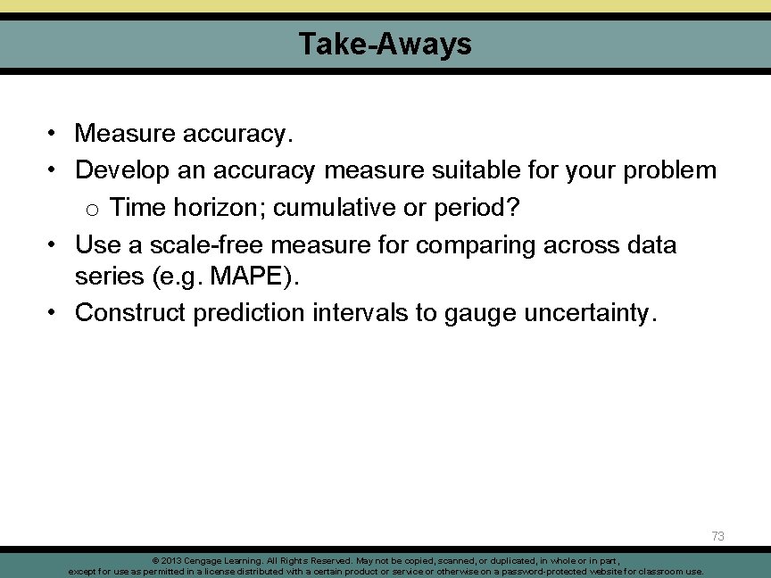
Take-Aways • Measure accuracy. • Develop an accuracy measure suitable for your problem o Time horizon; cumulative or period? • Use a scale-free measure for comparing across data series (e. g. MAPE). • Construct prediction intervals to gauge uncertainty. 73 © 2013 Cengage Learning. All Rights Reserved. May not be copied, scanned, or duplicated, in whole or in part, except for use as permitted in a license distributed with a certain product or service or otherwise on a password-protected website for classroom use.