2011 Pearson Education Inc Statistics for Business and

Statistics for Business and Economics Chapter 11 Multiple Regression and Model Building © 2011

Content 11. 1 Multiple Regression Models Part I: First-Order Models with Quantitative Independent Variables 11. 2 Estimating and Making Inferences about the Parameters 11. 3 Evaluating Overall Model Utility 11. 4 Using the Model for Estimation and Prediction © 2011 Pearson Education, Inc

Content Part II: Model Building in Multiple Regression 11. 5 Interaction Models 11. 6 Quadratic and Other Higher-Order Models 11. 7 Qualitative (Dummy) Variable Models 11. 8 Models with Both Quantitative and Qualitative Variables 11. 9 Comparing Nested Models © 2011 Pearson Education, Inc

Content 11. 10 Stepwise Regression Part III: Multiple Regression Diagnostics 11. 11 Residual Analysis: Checking the Regression Assumptions 11. 12 Some Pitfalls: Estimability, Multicollinearity, and Extrapolation © 2011 Pearson Education, Inc

Learning Objectives • • Introduce a multiple regression model as a means of relating a dependent variable y to two or more independent variables Present several different multiple regression models involving both quantitative and qualitative independent variables © 2011 Pearson Education, Inc

Learning Objectives • • Assess how well the multiple regression model fits the sample data Show an analysis of the model’s residuals can aid in detecting violations of model assumptions and in identifying model modifications © 2011 Pearson Education, Inc

11. 1 Multiple Regression Models © 2011 Pearson Education, Inc

The General Multiple Regression Model where y is the dependent variable. x 1, x 2, …, xk are the independent variables. E(y) = 0 + 1 x 1 + 2 x 2 +…+ kxk is the deterministic portion of the model. i determines the contribution of the independent variable xi. Note: The symbols x 1, x 2, …, xk may represent higherorder terms for quantitative predictors or terms that represent qualitative predictors. © 2011 Pearson Education, Inc

Analyzing a Multiple Regression Model Step 1 Hypothesize the deterministic component of the model. This component relates the mean, E(y), to the independent variables x 1, x 2, … , xk. This involves the choice of the independent variables to be included in the model. Step 2 Use the sample data to estimate the unknown model parameters 0, 1, 2, …, k in the model. © 2011 Pearson Education, Inc

Analyzing a Multiple Regression Model Step 3 Specify the probability distribution of the random error term, , and estimate the standard deviation of this distribution, . Step 4 Check that the assumptions on are satisfied and make model modifications if necessary. © 2011 Pearson Education, Inc

Analyzing a Multiple Regression Model Step 5 Statistically evaluate the usefulness of the model. Step 6 When satisfied that the model is useful, use it for prediction, estimation, and other purposes. © 2011 Pearson Education, Inc

Assumptions for Random Error For any given set of values of x 1, x 2, … , xk, the random error has a probability distribution with the following properties: 1. Mean equal to 0 2. Variance equal to 2 3. Normal distribution 4. Random errors are independent (in a probabilistic sense). © 2011 Pearson Education, Inc

Part I: First Order Models with Quantitative Independent Variables © 2011 Pearson Education, Inc

11. 2 Estimating and Making Inferences about the Parameter © 2011 Pearson Education, Inc

First-Order Model in Five Quantitative Independent (Predictor) Variables where x 1, x 2, … , x 5 are all quantitative variables that are not functions of other independent variables. Note: i represents the slope of the line relating y to xi when all the other x’s are held fixed. © 2011 Pearson Education, Inc

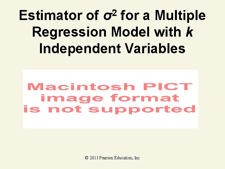
2 σ Estimator of for a Multiple Regression Model with k Independent Variables ©

Interpretation of Estimated Coefficients ^ 1. Slope ( k) • Estimated y changes by ^k for each 1 unit increase in xk holding all other variables constant 2. y-Intercept ( ^0) • Average value of y when xk = 0 © 2011 Pearson Education, Inc

Interpretation of Estimated Coefficients In first-order models, the relationship between E(y) and one of the variables, holding the others constant, will be a straight line and we get parallel straight lines as the values of the other variables change. © 2011 Pearson Education, Inc

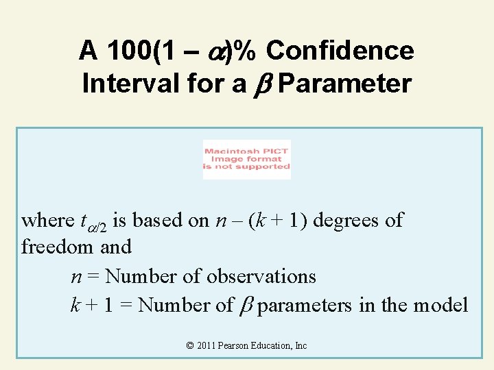
A 100(1 – )% Confidence Interval for a Parameter where t /2 is based on n – (k + 1) degrees of freedom and n = Number of observations k + 1 = Number of parameters in the model © 2011 Pearson Education, Inc

Test of an Individual Parameter Coefficient in the Multiple Regression Model One-Tailed Test H 0: i = 0 Ha: i < 0 (or Ha: i > 0) Rejection region: t < –t (or t > t when Ha: i > 0) where t is based on n – (k + 1) degrees of freedom n = Number of observations k + 1 = Number of parameters in the model © 2011 Pearson Education, Inc

Test of an Individual Parameter Coefficient in the Multiple Regression Model Two-Tailed Test H 0: i = 0 Ha : i ≠ 0 Rejection region: | t | > t where t /2 based on n – (k + 1) degrees of freedom n = Number of observations k + 1 = Number of parameters in the model © 2011 Pearson Education, Inc

Conditions Required for Valid Inferences about the Parameters For any given set of values of x 1, x 2, … , xk, the random error has a probability distribution with the following properties: 1. Mean equal to 0 2. Variance equal to 2 3. Normal distribution 4. Random errors are independent (in a probabilistic sense). © 2011 Pearson Education, Inc

First–Order Multiple Regression Model Relationship between 1 dependent and 2 or more independent variables is a linear function Population Y-intercept Dependent (response) variable Population slopes Random error Independent (explanatory) variables © 2011 Pearson Education, Inc

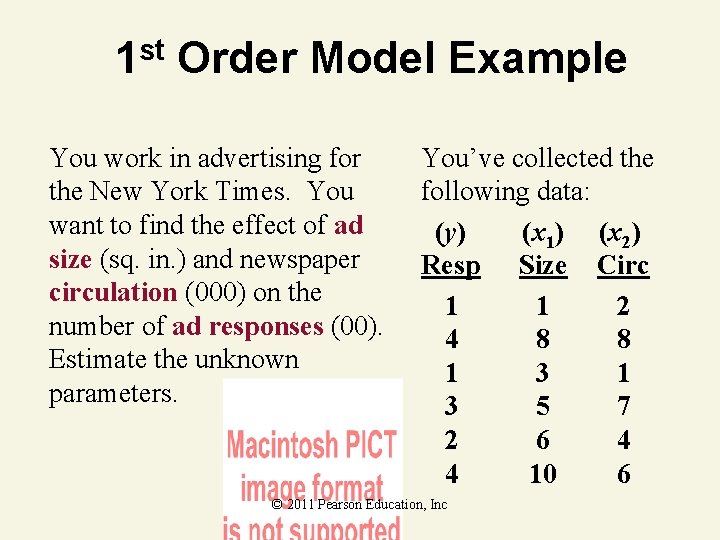
1 st Order Model Example You work in advertising for the New York Times. You want to find the effect of ad size (sq. in. ) and newspaper circulation (000) on the number of ad responses (00). Estimate the unknown parameters. You’ve collected the following data: (y) (x 1) (x 2) Resp Size Circ 1 1 2 4 8 8 1 3 5 7 2 6 4 4 10 6 © 2011 Pearson Education, Inc

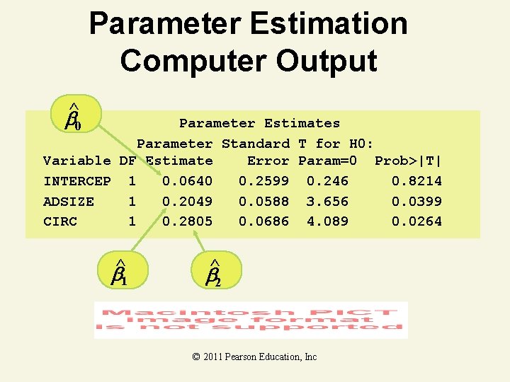
Parameter Estimation Computer Output ^0 Parameter Estimates Parameter Standard T for H 0: Variable DF Estimate Error Param=0 Prob>|T| INTERCEP 1 0. 0640 0. 2599 0. 246 0. 8214 ADSIZE 1 0. 2049 0. 0588 3. 656 0. 0399 CIRC 1 0. 2805 0. 0686 4. 089 0. 0264 ^1 ^2 © 2011 Pearson Education, Inc

Interpretation of Coefficients Solution ^ 1. Slope ( 1) • Number of responses to ad is expected to increase by 20. 49 for each 1 sq. increase in ad size holding circulation constant ^ 2. Slope ( 2) • Number of responses to ad is expected to increase by 28. 05 for each 1 unit (1, 000) increase in circulation holding ad size constant © 2011 Pearson Education, Inc

Calculating s 2 and s Example You work in advertising for the New York Times. You want to find the effect of ad size (sq. in. ), x 1, and newspaper circulation (000), x 2, on the number of ad responses (00), y. Find SSE, s 2, and s. © 2011 Pearson Education, Inc

Analysis of Variance Computer Output Analysis of Variance Source DF Regression 2 Residual Error 3 Total 5 SS 9. 249736. 250264 9. 5 MS 4. 624868. 083421 SSE © 2011 Pearson Education, Inc S 2 F 55. 44 P. 0043

11. 3 Evaluating Overall Model Utility © 2011 Pearson Education, Inc

Use Caution When Conducting t -tests on the Parameters It is dangerous to conduct t-tests on the individual parameters in a first-order linear model for the purpose of determining which independent variables are useful for predicting y and which are not. If you fail to reject H 0: i = 0, several conclusions are possible: 1. There is no relationship between y and xi. 2. A straight-line relationship between y and x exists (holding the other x’s in the model fixed), but a Type II error occurred. © 2011 Pearson Education, Inc

Use Caution When Conducting t -tests on the Parameters 3. A relationship between y and xi (holding the other x’s in the model fixed) exists but is more complex than a straight-line relationship (e. g. , a curvilinear relationship may be appropriate). The most you can say about a parameter test is that there is either sufficient (if you reject H 0: i = 0) or insufficient (if you do not reject H 0: i = 0) evidence of a linear (straight-line) relationship between y and xi. © 2011 Pearson Education, Inc

The Multiple Coefficient 2 of Determination, R is defined as © 2011 Pearson Education,

The Multiple Coefficient 2 of Determination, R • Proportion of variation in y ‘explained’ by all x variables taken together • Never decreases when new x variable is added to model — Only y values determine SSyy — Disadvantage when comparing models © 2011 Pearson Education, Inc

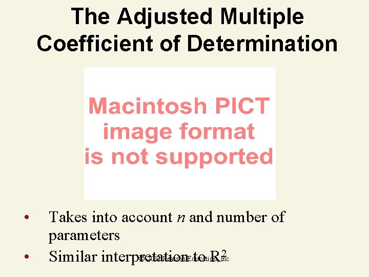
The Adjusted Multiple Coefficient of Determination • • Takes into account n and number

Estimation of R 2 and Ra 2 Example You work in advertising for the New York Times. You want to find the effect of ad size (sq. in. ), x 1, and newspaper circulation (000), x 2, on the number of ad responses (00), y. Find R 2 and Ra 2. © 2011 Pearson Education, Inc

Excel Computer Output Solution R 2 R a 2 © 2011 Pearson Education, Inc

Testing Global Usefulness of the Model: The analysis of Variance F-Test H 0: 1 = 2 = … = k = 0 (All model terms are unimportant for predicting y) Ha: At least one i ≠ 0 (At least one model term is useful for predicting y) © 2011 Pearson Education, Inc

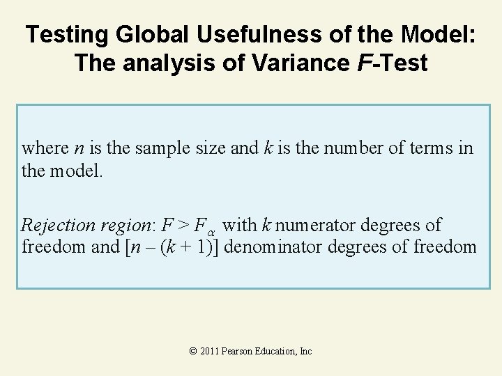
Testing Global Usefulness of the Model: The analysis of Variance F-Test where n is the sample size and k is the number of terms in the model. Rejection region: F > F with k numerator degrees of freedom and [n – (k + 1)] denominator degrees of freedom © 2011 Pearson Education, Inc

Recommendation for Checking the Utility of a Multiple Regression Model 1. First, conduct a test of overall model adequacy using the F-test–that is, test H 0: 1 = 2 =…= k = 0 If the model is deemed adequate (that is, if you reject H 0), then proceed to step 2. Otherwise, you should hypothesize and fit another model. The new model may include more independent variables or higher-order terms. © 2011 Pearson Education, Inc

Recommendation for Checking the Utility of a Multiple Regression Model 2. Conduct t-tests on those parameters in which you are particularly interested (that is, the “most important” ’s). These usually involve only the ’s associated with higher-order terms (x 2, x 1 x 2, etc. ). However, it is a safe practice to limit the number of ’s that are tested. Conducting a series of t-tests leads to a high overall Type I error rate . © 2011 Pearson Education, Inc

Testing Overall Significance Example You work in advertising for the New York Times. You want to find the effect of ad size (sq. in. ), x 1, and newspaper circulation (000), x 2, on the number of ad responses (00), y. Conduct the global F–test of model usefulness. Use α =. 05. © 2011 Pearson Education, Inc

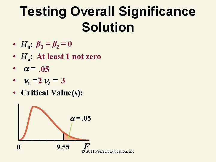
Testing Overall Significance Solution H 0: β 1 = β 2 = 0 Ha:

Testing Overall Significance Computer Output k Source DF Model 2 Error 3 C Total 5 Analysis of Variance Sum of Squares 9. 2497 0. 2503 9. 5000 n – (k + 1) Mean Square 4. 6249 0. 0834 F Value 55. 440 Prob>F 0. 0043 MS(Model) MS(Error) © 2011 Pearson Education, Inc

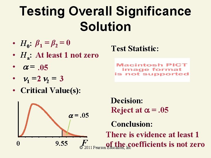
Testing Overall Significance Solution H 0: β 1 = β 2 = 0 Ha: At least 1 not zero =. 05 1 = 2 2 = 3 Critical Value(s): • • • =. 05 0 9. 55 Test Statistic: Decision: Reject at =. 05 Conclusion: There is evidence at least 1 F the. Inccoefficients is not zero © 2011 Pearsonof Education,

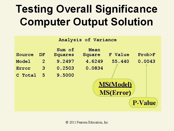
Testing Overall Significance Computer Output Solution Analysis of Variance Source DF Model 2 Error 3 C Total 5 Sum of Squares 9. 2497 0. 2503 9. 5000 Mean Square 4. 6249 0. 0834 F Value 55. 440 Prob>F 0. 0043 MS(Model) MS(Error) P-Value © 2011 Pearson Education, Inc

11. 4 Using the Model for Estimation and Prediction © 2011 Pearson Education, Inc

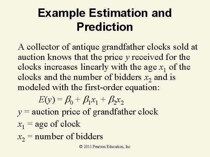
Example Estimation and Prediction A collector of antique grandfather clocks sold at auction knows that the price y received for the clocks increases linearly with the age x 1 of the clocks and the number of bidders x 2 and is modeled with the first-order equation: E(y) = 0 + 1 x 1 + 2 x 2 y = auction price of grandfather clock x 1 = age of clock x 2 = number of bidders © 2011 Pearson Education, Inc

Example Estimation and Prediction © 2011 Pearson Education, Inc

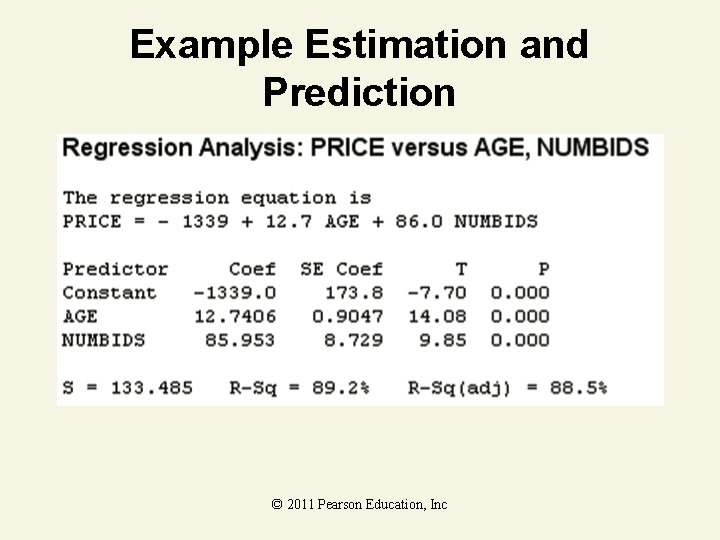
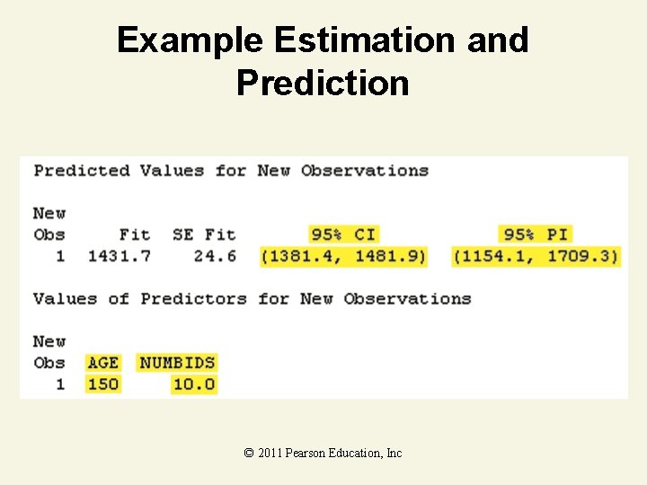
Example Estimation and Prediction a. Estimate the average auction price for all 150 year-old clocks sold at auctions with 10 bidders using a 95% confidence interval. Interpret the result. Here, the key words average and for all imply we want to estimate the mean of y, E(y). We want a 95% confidence interval for E(y) when x 1 = 150 years and x 2 = 10 bidders. A Minitab printout for this analysis is shown. . . © 2011 Pearson Education, Inc

Example Estimation and Prediction The confidence interval (highlighted under “ 95% CI”) is (1, 381. 4, 1, 481. 9). Thus, we are 95% confident that the mean auction price for all 150 year-old clocks sold at an auction with 10 bidders lies between $1, 381. 40 and $1, 481. 90. © 2011 Pearson Education, Inc

Example Estimation and Prediction b. Predict the auction price for a single 150 -year old clock sold at an auction with 10 bidders using a 95% prediction interval. Interpret the result. The key words predict and for a single imply that we want a 95% prediction interval for y when x 1 = 150 years and x 2 = 10 bidders. This interval (highlighted under “ 95% PI” on the Minitab printout) is (1, 154. 1, 1, 709. 3). We say, with 95% confidence, that the auction price for a single 150 year-old clock sold at an auction with 10 bidders © 2011 Pearson Education, Inc falls between $1, 154. 10 and $1, 709. 30.

Example Estimation and Prediction c. Suppose you want to predict the auction price for one clock that is 50 years old and has 2 bidders. How should you proceed? Now, we want to predict the auction price, y, for a single (one) grandfather clock when x 1 = 50 years and x 2 = 2 bidders. Consequently, we desire a 95% prediction interval for y. However, before we form this prediction interval, we should check to make sure that the selected values of the independent variables, x 1 = 50 and x 2 = 2, are both reasonable © 2011 Pearson Education, Inc and within their respective sample ranges.

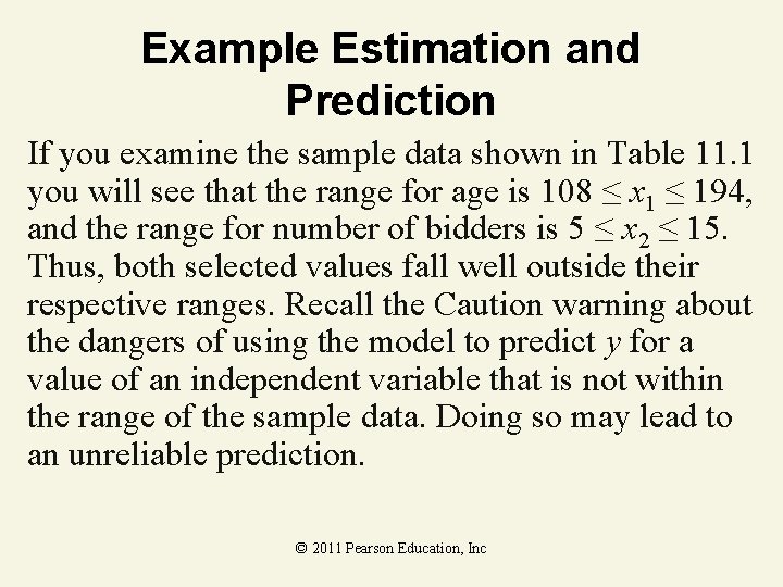
Example Estimation and Prediction If you examine the sample data shown in Table 11. 1 you will see that the range for age is 108 ≤ x 1 ≤ 194, and the range for number of bidders is 5 ≤ x 2 ≤ 15. Thus, both selected values fall well outside their respective ranges. Recall the Caution warning about the dangers of using the model to predict y for a value of an independent variable that is not within the range of the sample data. Doing so may lead to an unreliable prediction. © 2011 Pearson Education, Inc

Part II: Model Building in Multiple Regression © 2011 Pearson Education, Inc

11. 5 Interaction Models © 2011 Pearson Education, Inc

An Interaction Model Relating E(y) to Two Quantitative Independent Variables where ( 1 + 3 x 2) represents the change in E(y) for every 1 -unit increase in x 1, holding x 2 fixed ( 2 + 3 x 1) represents the change in E(y) for every 1 -unit increase in x 2, holding x 1 fixed © 2011 Pearson Education, Inc

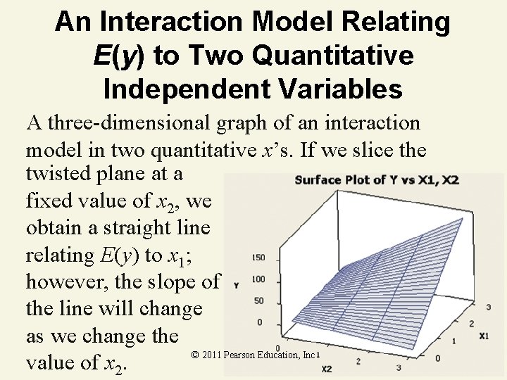
An Interaction Model Relating E(y) to Two Quantitative Independent Variables A three-dimensional graph of an interaction model in two quantitative x’s. If we slice the twisted plane at a fixed value of x 2, we obtain a straight line relating E(y) to x 1; however, the slope of the line will change as we change the © 2011 Pearson Education, Inc value of x 2.

Interaction Model With 2 Independent Variables • Hypothesizes interaction between pairs of x variables — Response to one x variable varies at different levels of another x variable • Contains two-way cross product terms • Can be combined with other models — Example: dummy-variable model © 2011 Pearson Education, Inc

Effect of Interaction Given: • Without interaction term, effect of x 1 on y is measured by 1 • With interaction term, effect of x 1 on y is measured by 1 + 3 x 2 — Effect increases as x 2 increases © 2011 Pearson Education, Inc

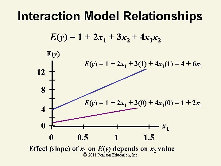
Interaction Model Relationships E(y) = 1 + 2 x 1 + 3 x 2 + 4 x 1 x 2 E(y) = 1 + 2 x 1 + 3(1) + 4 x 1(1) = 4 + 6 x 1 12 8 E(y) = 1 + 2 x 1 + 3(0) + 4 x 1(0) = 1 + 2 x 1 4 x 1 0 0 0. 5 1 1. 5 Effect (slope) of x 1 on E(y) depends on x 2 value © 2011 Pearson Education, Inc

Interaction Example You work in advertising for the New York Times. You want to find the effect of ad size (sq. in. ), x 1, and newspaper circulation (000), x 2, on the number of ad responses (00), y. Conduct a test for interaction. Use α =. 05. © 2011 Pearson Education, Inc

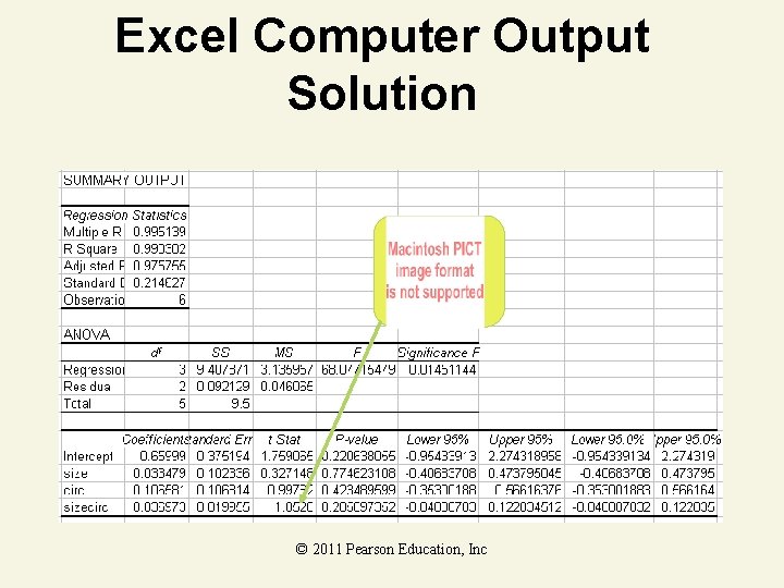
Excel Computer Output Solution Global F–test indicates at least one parameter is not zero

Interaction Test Solution • • • H 0: 3 = 0 Ha: 3 ≠

Excel Computer Output Solution © 2011 Pearson Education, Inc

Interaction Test Solution • • • H 0: 3 = 0 Ha: 3 ≠ 0 . 05 df 6 – 4 = 2 Critical Value(s): Reject H 0. 025 – 4. 303 Reject H 0. 025 0 4. 303 Test Statistic: t = 1. 8528 Decision: Do no reject at =. 05 Conclusion: There is no evidence of t interaction © 2011 Pearson Education, Inc

11. 6 Quadratic and Other Higher-Order Models © 2011 Pearson Education, Inc

A Quadratic (Second-Order) Model in a Single Quantitative Independent Variable where 0 is the y-intercept of the curve. 1 is a shift parameter. 2 is the rate of curvature. © 2011 Pearson Education, Inc

Second-Order Model Relationships y 2 > 0 x 1 y 2 < 0 x

2 nd Order Model Example The data shows the number of weeks employed and the number of errors made per day for a sample of assembly line workers. Find a 2 nd order model, conduct the global F–test, and test if β 2 ≠ 0. Use α =. 05 for all tests. © 2011 Pearson Education, Inc Errors (y) 20 18 16 10 8 4 3 1 2 1 0 1 Weeks (x) 1 1 2 4 4 5 6 8 10 11 12 12

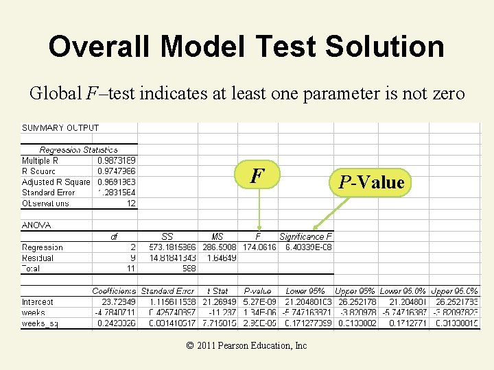
Overall Model Test Solution Global F–test indicates at least one parameter is not zero

β 2 Parameter Test Solution β 2 test indicates curvilinear relationship exists t P-Value

A Complete Second-Order Model with Two Quantitative Independent Variables Comments on the Parameters 0 : y-intercept, the value of E(y) when x 1 = x 2 = 0 1: 2 changing 1 and 2 causes the surface to shift along the x 1 - and x 2 -axes 3: controls the rotation of the surface 4: 5 signs and values of these parameters control © 2011 Pearson Inc the type of surface and. Education, the rates of curvature

Second-Order Model Relationships y x 2 x 1 y x 1 4 + 5

11. 7 Qualitative (Dummy) Variable Models © 2011 Pearson Education, Inc

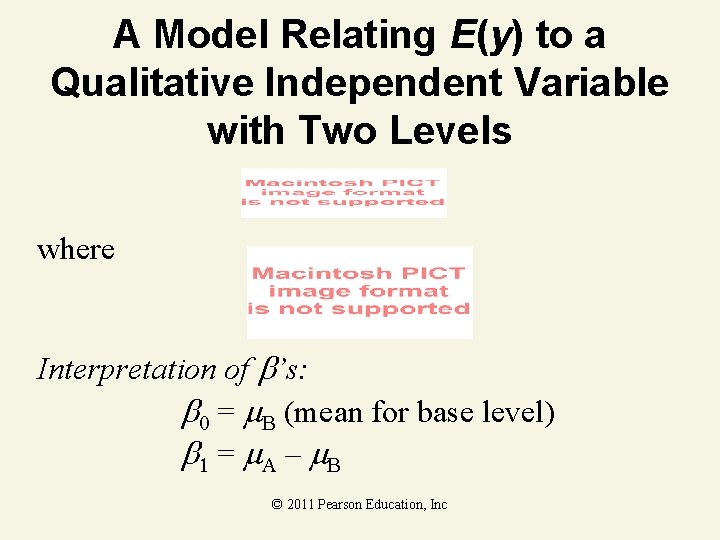
A Model Relating E(y) to a Qualitative Independent Variable with Two Levels where Interpretation

Dummy-Variable Model • Involves categorical x variable with 2 levels — e. g. , male-female; college-no college • • • Variable levels coded 0 and 1 Number of dummy variables is 1 less than number of levels of variable May be combined with quantitative variable (1 st order or 2 nd order model) © 2011 Pearson Education, Inc

Interpreting Dummy. Variable Model Equation Given: y = Starting salary of college graduates x 1 = GPA 0 if Male x 2 = 1 if Female Same slopes Male ( x 2 = 0 ): Female ( x 2 = 1 ): © 2011 Pearson Education, Inc

Dummy-Variable Model Example Computer Output: 0 if Male x 2 = 1 if Female

Dummy-Variable Model Relationships y Same Slopes ^1 Female ^ + ^ 0 2 Male

A Model Relating E(y) to One Qualitative Independent Variable with k Levels where xi is the dummy variable for level i + 1 and Then, for this system of coding A = C = + B = + D = + © 2011 Pearson Education, Inc B A C A D A

11. 8 Models with Both Quantitative and Qualitative Variables © 2011 Pearson Education, Inc

Example Substitute the appropriate values of the dummy variables in the model to obtain

Example The complete model that characterizes the three lines in the figure is where

Example Examining the coding, you can see that x 2 = x 3 = 0 when the advertising medium is newspaper. Substituting these values into the expression for E(y), we obtain the newspaper medium line: © 2011 Pearson Education, Inc

Example Similarly, we substitute the appropriate values of x 2 and x 3 into

Example and the television medium line: (x 2 = 0, x 3 = 1):

Example Why bother fitting a model that combines all three lines (model 3) into the same equation? The answer is that you need to use this procedure if you wish to use statistical tests to compare three media lines. We need to be able to express a practical question about the lines in terms of a hypothesis that a set of parameters in the model equals 0. You could not do this if you were to perform three separate regression analyses and fit a line to each set of media data. © 2011 Pearson Education, Inc

11. 9 Comparing Nested Models © 2011 Pearson Education, Inc

Nested Models Two models are nested if one model contains all the terms of the second model and at least one additional term. The more complex of the two models is called the complete (or full) model, and the simpler of the two is called the reduced model. © 2011 Pearson Education, Inc

Comparing Nested Models • • • Contains a subset of terms in the complete (full) model Tests the contribution of a set of x variables to the relationship with y Null hypothesis H 0: g+1 =. . . = k = 0 — Variables in set do not improve significantly the model when all other variables are included Used in selecting x variables or models Part of most computer programs © 2011 Pearson Education, Inc

F-Test for Comparing Nested Models Reduced model: Complete model: Ha: At least one of

F-Test for Comparing Nested Models Test statistic: © 2011 Pearson Education, Inc

F-Test for Comparing Nested Models where SSER = Sum of squared errors for the reduced model SSEC = Sum of squared errors for the complete model MSEC = Mean square error (s 2)for the complete model k – g = Number of parameters specified in H 0 (i. e. , number of parameters tested) © 2011 Pearson Education, Inc

F-Test for Comparing Nested Models where k +1 = Number of parameters in the complete model (including 0) n = total sample size Rejection region: F > F Where F is based on v 1 = k – g numerator degrees of freedom and v 2 = n – (k + 1) denominator degrees of freedom. © 2011 Pearson Education, Inc

Parsimonious Models A parsimonious model is a general linear model with a small number of parameters. In situations where two competing models have essentially the same predictive power (as determined by an F-test), choose the more parsimonious of the two. © 2011 Pearson Education, Inc

Guidelines for Selecting Preferred Model in a Nested Model F-Test Conclusion Preferred Model Reject

11. 10 Stepwise Regression © 2011 Pearson Education, Inc

Stepwise Regression The user first identifies the response, y, and the set of potentially important independent variables, x 1, x 2, … , xk, where k is generally large. The response and independent variables are then entered into the computer software, and the stepwise procedure begins. © 2011 Pearson Education, Inc

Stepwise Regression Step 1 Software program fits all possible onevariable models of the form E(y) = 0 + 1 x 1 to the data, where xi is the ith independent variable, i = 1, 2, … , k. Test the null hypothesis H 0: 1 = 0 against the alternative Ha: 1 ≠ 0. The independent variable that produces the largest (absolute) t-value is declared the best one-variable predictor of y: x 1 © 2011 Pearson Education, Inc

Stepwise Regression Step 2 The stepwise program now begins to search through the remaining (k – 1) independent variables for the best twovariable model of the form E(y) = 0 + 1 x 1 + 2 xi Again the variable having the largest t value is retained: x 2 © 2011 Pearson Education, Inc

Stepwise Regression Step 3 The stepwise procedure now checks for a third independent variable to include in the model with x 1 and x 2 –that is, we seek the best model of the form E(y) = 0 + 1 x 1 + 2 x 2 + 3 xi Again the variable having the largest t value is retained: x 3 © 2011 Pearson Education, Inc

Stepwise Regression The result of the stepwise procedure is a model containing only those terms with t-values that are significant at the specified level. Thus, in most practical situations, only several of the large number of independent variables remain. We have very probably included some unimportant independent variables in the model (Type I errors) and eliminated some important ones (Type II errors). © 2011 Pearson Education, Inc

Stepwise Regression There is a second reason why we might not have arrived at a good model. When we choose the variables to be included in the stepwise regression, we may often omit higher-order terms (to keep the number of variables manageable). Consequently, we may have initially omitted several important terms from the model. Thus, we should recognize stepwise regression for what it is: an objective variable screening procedure. © 2011 Pearson Education, Inc

Part III: Multiple Regression Diagnostics © 2011 Pearson Education, Inc

11. 11 Residual Analysis: Checking the Regression Assumptions © 2011 Pearson Education, Inc

Regression Residual A regression residual, , is defined as the difference between an observed

Properties of Regression Residual 1. The mean of the residuals is equal to 0. This property follows from the fact that the sum of the differences between the observed y values and their least squares predicted values is equal to 0. © 2011 Pearson Education, Inc

Properties of Regression Residual 2. The standard deviation of the residuals is equal to the standard deviation of the fitted regression model, s. This property follows from the fact that the sum of the squared residuals is equal to SSE, which when divided by the error degrees of freedom is equal to the variance of the fitted regression model, s 2. © 2011 Pearson Education, Inc

Properties of Regression Residual 2. The square root of the variance is both the

Regression Outlier A regression outlier is a residual that is larger than 3 s

Residual Analysis • Graphical analysis of residuals — Plot estimated errors versus xi values — Plot histogram or stem-&-leaf of residuals • Purposes — Examine functional form (linear v. non-linear model) — Evaluate violations of assumptions © 2011 Pearson Education, Inc

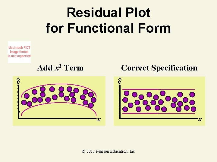
Residual Plot for Functional Form Add x 2 Term Correct Specification ^ e ^e

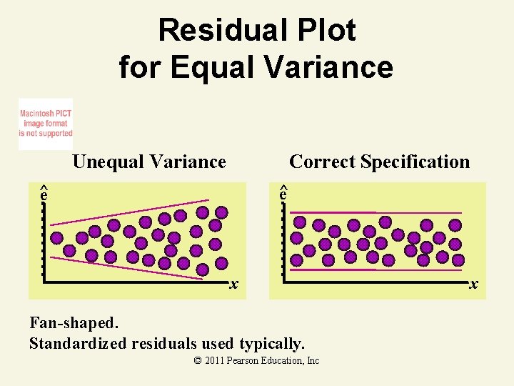
Residual Plot for Equal Variance Unequal Variance Correct Specification ^ e x Fan-shaped. Standardized

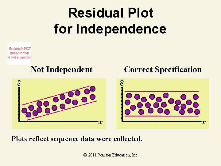
Residual Plot for Independence Not Independent Correct Specification ^ e x Plots reflect sequence

Residual Analysis Computer Output Dep Var Predict Student Obs SALES Value Residual -2 -1 -0 1 2 1 1. 0000 0. 6000 0. 4000 1. 044 | |** 2 1. 0000 1. 3000 -0. 592 | *| 3 2. 0000 0 0. 000 | | 4 2. 0000 2. 7000 -0. 7000 -1. 382 | **| 5 4. 0000 3. 4000 0. 6000 1. 567 | |*** Plot of standardized (student) residuals © 2011 Pearson Education, Inc | | |

Steps in a Residual Analysis 1. Check for a misspecified model by plotting the residuals against each of the quantitative independent variables. Analyze each plot, looking for a curvilinear trend. This shape signals the need for a quadratic term in the model. Try a second-order term in the variable against which the residuals are plotted. © 2011 Pearson Education, Inc

Steps in a Residual Analysis 2. Examine the residual plots for outliers. Draw lines on the residual plots at 2 - and 3 -standard -deviation distances below and above the 0 line. Examine residuals outside the 3 -standard -deviation lines as potential outliers and check to see that no more than 5% of the residuals exceed the 2 -standard-deviation lines. Determine whether each outlier can be explained as an error in data collection or transcription, corresponds ot a member of a © 2011 Pearson Education, Inc

Steps in a Residual Analysis 2. population different from that of the remainder of the sample, or simply represents an unusual observation. If the observation is determined to be an error, fix it or remove it. Even if you cannot determine the cause, you may want to rerun the regression analysis without the observation to determine its effect on the analysis. © 2011 Pearson Education, Inc

Steps in a Residual Analysis 3. Check for nonnormal errors by plotting a frequency distribution of the residuals, using a stem-and-leaf display or a histogram. Check to see if obvious departures from normality exist. Extreme skewness of the frequency distribution may be due to outliers or could indicate the need for a transformation of the dependent variable. (Normalizing transformations are beyond the scope of this book, but you can find information in the references. ) © 2011 Pearson Education, Inc

Steps in a Residual Analysis 4. Check for unequal error variances by plotting the residuals against the predicted values, . If you detect a cone-shaped pattern or some other pattern that indicates that the variance of is not constant, refit the model using an appropriate variance-stabilizing transformation on y, such as ln(y). (Consult the references for other useful variancestabilizing transformations. ) © 2011 Pearson Education, Inc

11. 12 Some Pitfalls: Estimability, Multicollinearity, and Extrapolation © 2011 Pearson Education, Inc

Regression Pitfalls • Parameter Estimability — Number of levels of observed x–values must be one more than order of the polynomial in x • Multicollinearity — Two or more x–variables in the model are correlated • Extrapolation — Predicting y–values outside sampled range • Correlated Errors © 2011 Pearson Education, Inc

Multicollinearity • • • High correlation between x variables Coefficients measure combined effect Leads to unstable coefficients depending on x variables in model Always exists – matter of degree Example: using both age and height as explanatory variables in same model © 2011 Pearson Education, Inc

Detecting Multicollinearity • • • Significant correlations between pairs of independent variables Nonsignificant t–tests for all of the individual parameters when the F-test for overall model adequacy is significant Sign opposite from what is expected in the estimated parameters © 2011 Pearson Education, Inc

Using the Correlation Coefficient r to Detect Multicollinearity • • • Extreme multicollinearity: | r | ≥. 8 Moderate multicollinearity: . 2 ≤ | r | <. 8 Low multicollinearity: | r | <. 2 © 2011 Pearson Education, Inc

Solutions to Some Problems Created by Multicollinearity in Regression 1. Drop one or more of the correlated independent variables from the model. One way to decide which variables to keep in the model is to employ stepwise regression. © 2011 Pearson Education, Inc

Solutions to Some Problems Created by Multicollinearity in Regression 2. If you decide to keep all the independent variables in the model, a. Avoid making inferences about the individual parameters based on the t-tests. b. Restrict inferences about E(y) and future y values to values of the x’s that fall within the range of the sample data. © 2011 Pearson Education, Inc

Extrapolation y Interpolation Extrapolation Sampled Range © 2011 Pearson Education, Inc x

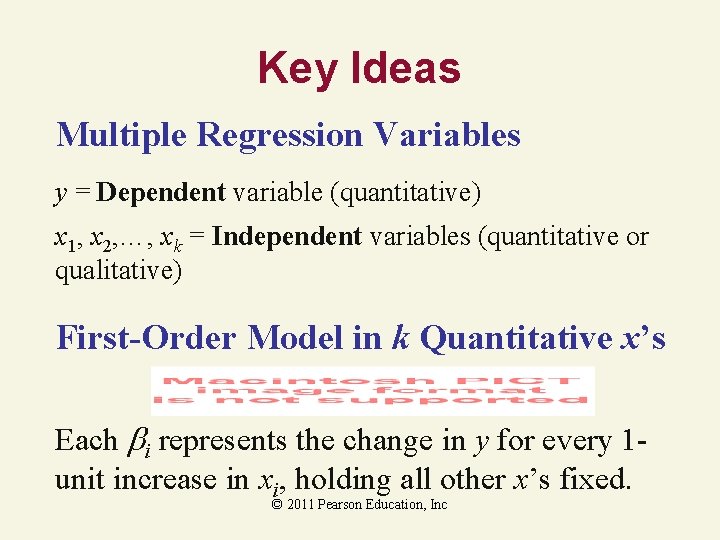
Key Ideas Multiple Regression Variables y = Dependent variable (quantitative) x 1, x 2, …, xk = Independent variables (quantitative or qualitative) First-Order Model in k Quantitative x’s Each i represents the change in y for every 1 unit increase in xi, holding all other x’s fixed. © 2011 Pearson Education, Inc

Key Ideas Interaction Model in 2 Quantitative x’s ( 1 + 3 x 2) represents the change in y for every 1 -unit increase in x 1, for fixed value of x 2 ( 2 + 3 x 1) represents the change in y for every 1 -unit increase in x 2, for fixed value of x 1 © 2011 Pearson Education, Inc

Key Ideas Quadratic Model in 1 Quantitative x 2 represents the rate of curvature

Key Ideas Complete Second-Order Model in 2 Quantitative x’s 4 represents the rate of curvature in y for x 1, holding x 2 fixed 5 represents the rate of curvature in y for x 2, holding x 1 fixed © 2011 Pearson Education, Inc

Key Ideas Dummy Variable Model for k Qualitative x x 1 = {1 if level 1, 0 if not} x 2 = {1 if level 1, 0 if not} xk – 1 = {1 if level 1, 0 if not} 0 = E(y) for level k (base level) = k 1 = 1 – k 2 = 2 – k © 2011 Pearson Education, Inc

Key Ideas Complete Second-Order Model in 1 Quantitative x and 1 Qualitative x (Two

Key Ideas Adjusted Coefficient of Determination Cannot be “forced” to 1 by adding independent variables to the model. Interaction between x 1 and x 2 Implies that the relationship between y and one x depends on the other x. Parsimonious Model A model with a small number of parameters. © 2011 Pearson Education, Inc

Key Ideas Recommendation for Assessing Model Adequacy 1. Conduct global F-test; if significant then: 2. Conduct t-tests on only the most important ’s (interaction or squared terms) 3. Interpret value of 2 s 4. Interpret value of © 2011 Pearson Education, Inc

Key Ideas Recommendation for Testing Individual ’s 1. If curvature (x 2) deemed important, do not conduct test for first-order (x) term in the model. 2. If interaction (x 1 x 2) deemed important, do not conduct tests for first-order terms (x 1 and x 2) in the model. © 2011 Pearson Education, Inc

Key Ideas Extrapolation Occurs when you predict y for values of x’s that are outside of range of sample data. Nested Models Are models where one model (the complete model) contains all the terms of another model (the reduced model) plus at least one additional term. © 2011 Pearson Education, Inc

Key Ideas Multicollinearity Occurs when two or more x’s are correlated. Indicators of multicollinearity: 1. Highly correlated x’s 2. Significant, global F-test, but all t-tests nonsignificant 3. Signs on ’s opposite from expected © 2011 Pearson Education, Inc

Key Ideas Problems with Using Stepwise Regression Model as the “Final” Model 1. Extremely large number of t-tests inflate overall probability of at least one Type I error. 2. No higher-order terms (interactions or squared terms) are included in the model. © 2011 Pearson Education, Inc

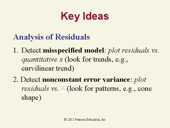
Key Ideas Analysis of Residuals 1. Detect misspecified model: plot residuals vs. quantitative x (look for trends, e. g. , curvilinear trend) 2. Detect nonconstant error variance: plot residuals vs. (look for patterns, e. g. , cone shape) © 2011 Pearson Education, Inc

Key Ideas Analysis of Residuals 3. Detect nonnormal errors: histogram, stemleaf, or normal probability plot of residuals (look for strong departures from normality) 4. Identify outliers: residuals greater than 3 s in absolute value (investigate outliers before deleting) © 2011 Pearson Education, Inc