2011 Pearson Education Inc Statistics for Business and

Statistics for Business and Economics Chapter 13 Time Series: Descriptive Analyses, Models, & Forecasting

Content 13. 1 Descriptive Analysis: Index Numbers 13. 2 Descriptive Analysis: Exponential Smoothing 13. 3 Time Series Components 13. 4 Forecasting: Exponential Smoothing 13. 5 Forecasting Trends: Holt’s Method 13. 6 Measuring Forecast Accuracy: MAD and RMSE © 2011 Pearson Education, Inc

Content 13. 7 Forecasting Trends: Simple Linear Regression 13. 8 Seasonal Regression Models 13.

Learning Objectives • • • Focus on methods for analyzing data generated by a process over time (i. e. , time series data). Present descriptive methods for characterizing time series data. Present inferential methods forecasting future values of time series data. © 2011 Pearson Education, Inc

Time Series • Data generated by processes over time • Describe and predict output of processes • Descriptive analysis – Understanding patterns • Inferential analysis – Forecast future values © 2011 Pearson Education, Inc

13. 1 Descriptive Analysis: Index Numbers © 2011 Pearson Education, Inc

Index Number • Measures change over time relative to a base period • Price Index measures changes in price – e. g. Consumer Price Index (CPI) • Quantity Index measures changes in quantity – e. g. Number of cell phones produced annually © 2011 Pearson Education, Inc

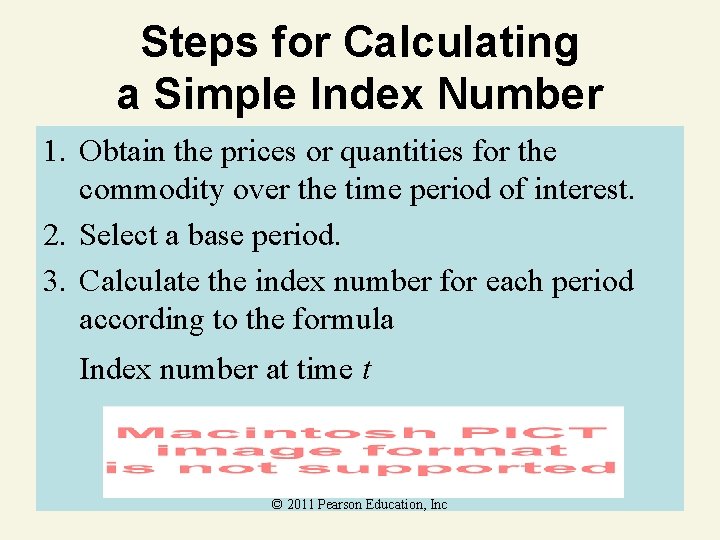
Steps for Calculating a Simple Index Number 1. Obtain the prices or quantities for the commodity over the time period of interest. 2. Select a base period. 3. Calculate the index number for each period according to the formula Index number at time t © 2011 Pearson Education, Inc

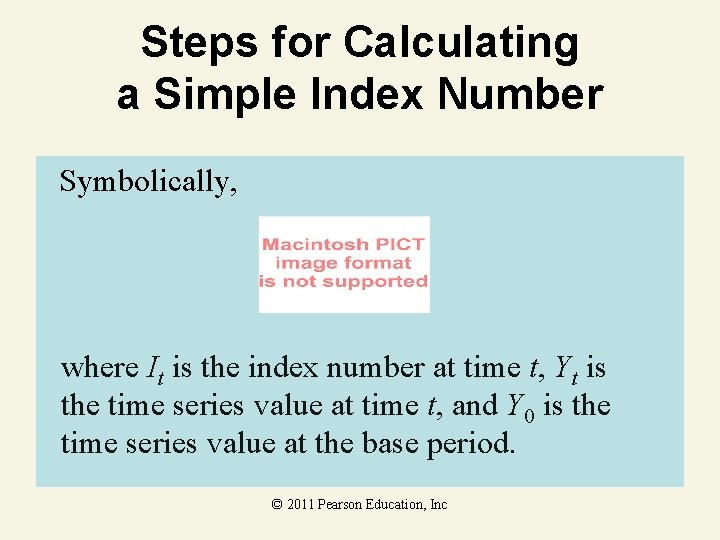
Steps for Calculating a Simple Index Number Symbolically, where It is the index number at time t, Yt is the time series value at time t, and Y 0 is the time series value at the base period. © 2011 Pearson Education, Inc

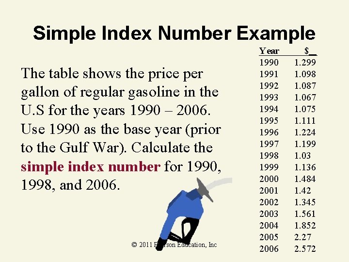
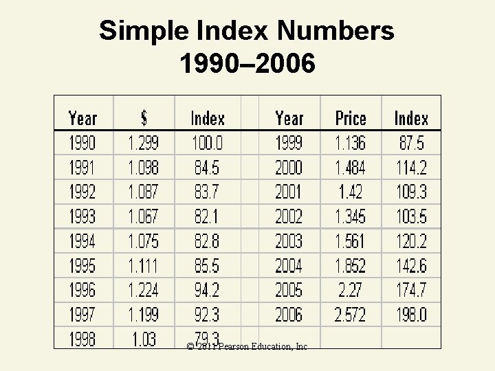
Simple Index Number Example The table shows the price per gallon of regular gasoline in the U. S for the years 1990 – 2006. Use 1990 as the base year (prior to the Gulf War). Calculate the simple index number for 1990, 1998, and 2006. © 2011 Pearson Education, Inc Year 1990 1991 1992 1993 1994 1995 1996 1997 1998 1999 2000 2001 2002 2003 2004 2005 2006 $ 1. 299 1. 098 1. 087 1. 067 1. 075 1. 111 1. 224 1. 199 1. 03 1. 136 1. 484 1. 42 1. 345 1. 561 1. 852 2. 27 2. 572

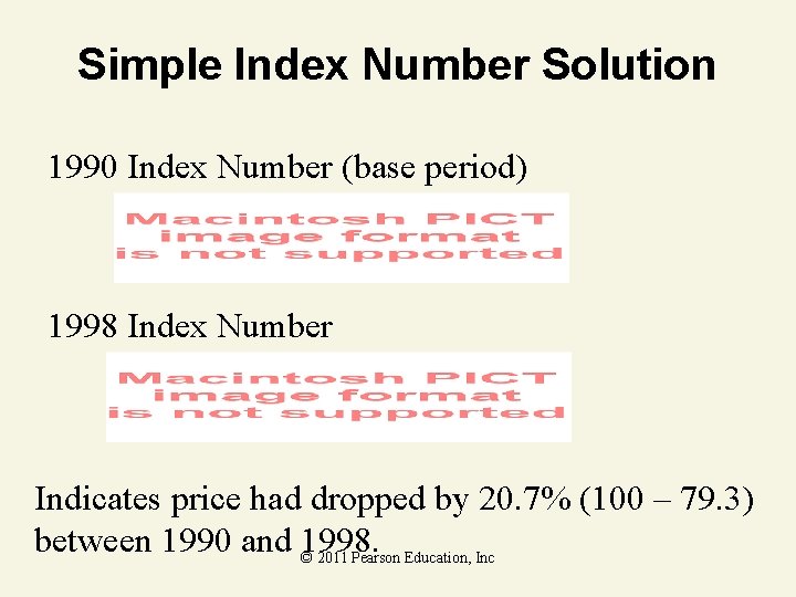
Simple Index Number Solution 1990 Index Number (base period) 1998 Index Number Indicates price

Simple Index Number Solution 2006 Index Number Indicates price had risen by 98% (100

Simple Index Numbers 1990– 2006 © 2011 Pearson Education, Inc

Composite Index Number • Made up of two or more commodities • A simple index using the total price or total quantity of all the series (commodities) • Disadvantage: Quantity of each commodity purchased is not considered © 2011 Pearson Education, Inc

Composite Index Number Example The table on the next slide shows the closing stock prices on the last day of the month for Daimler–Chrysler, Ford, and GM between 2005 and 2006. Construct the simple composite index using January 2005 as the base period. (Source: Nasdaq. com) © 2011 Pearson Education, Inc

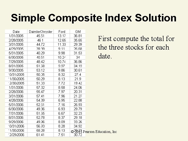
Simple Composite Index Solution First compute the total for the three stocks for each

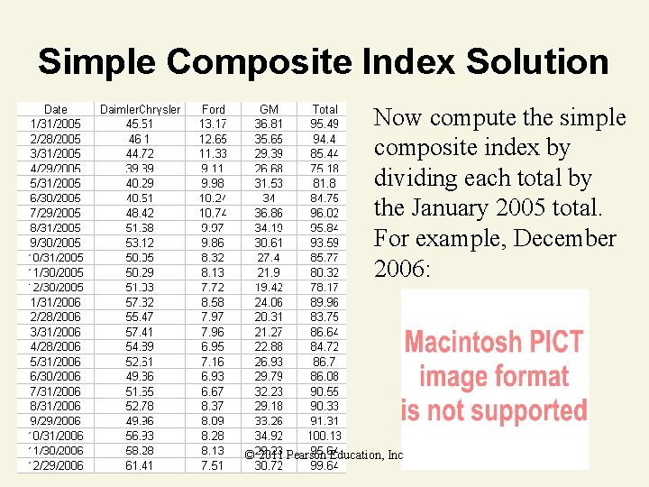
Simple Composite Index Solution Now compute the simple composite index by dividing each total

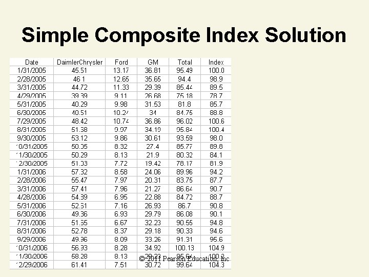
Simple Composite Index Solution © 2011 Pearson Education, Inc

Weighted Composite Price Index A weighted composite price index weights the prices by quantities purchased prior to calculating totals for each time period. The weighted totals are then used to compute the index in the same way that the unweighted totals are used for simple composite indexes. © 2011 Pearson Education, Inc

Laspeyres Index • Uses base period quantities as weights – Appropriate when quantities remain approximately constant over time period • Example: Consumer Price Index (CPI) © 2011 Pearson Education, Inc

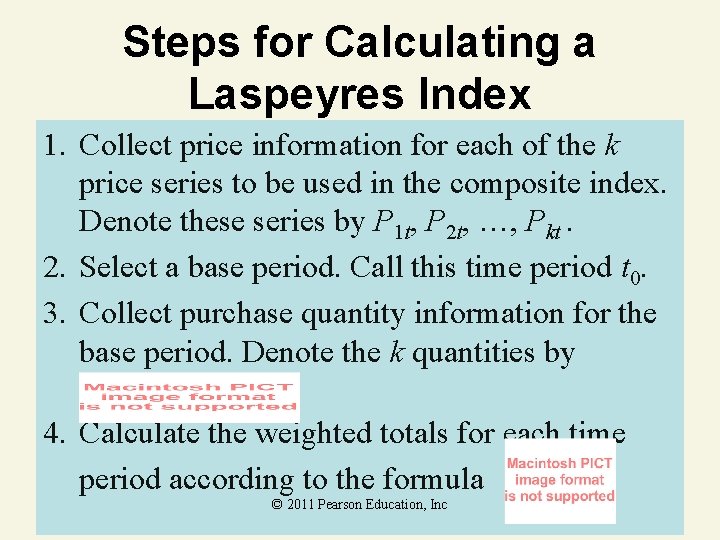
Steps for Calculating a Laspeyres Index 1. Collect price information for each of the k price series to be used in the composite index. Denote these series by P 1 t, P 2 t, …, Pkt. 2. Select a base period. Call this time period t 0. 3. Collect purchase quantity information for the base period. Denote the k quantities by 4. Calculate the weighted totals for each time period according to the formula © 2011 Pearson Education, Inc

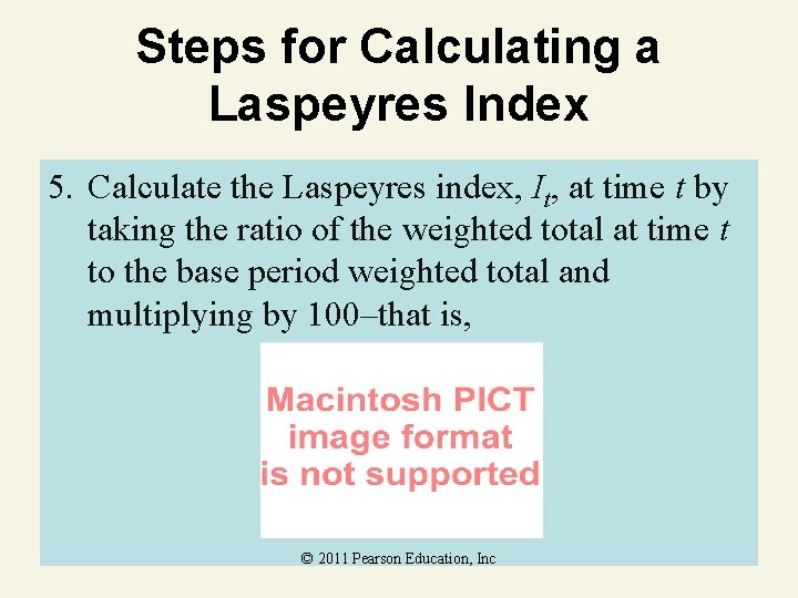
Steps for Calculating a Laspeyres Index 5. Calculate the Laspeyres index, It, at time t by taking the ratio of the weighted total at time t to the base period weighted total and multiplying by 100–that is, © 2011 Pearson Education, Inc

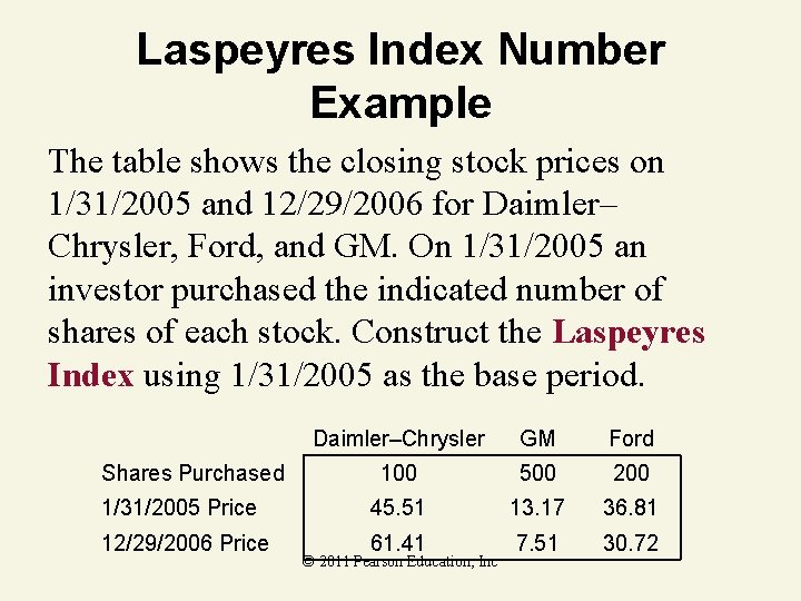
Laspeyres Index Number Example The table shows the closing stock prices on 1/31/2005 and 12/29/2006 for Daimler– Chrysler, Ford, and GM. On 1/31/2005 an investor purchased the indicated number of shares of each stock. Construct the Laspeyres Index using 1/31/2005 as the base period. Daimler–Chrysler GM Ford 100 500 200 1/31/2005 Price 45. 51 13. 17 36. 81 12/29/2006 Price 61. 41 7. 51 30. 72 Shares Purchased © 2011 Pearson Education, Inc

Laspeyres Index Solution Weighted total for base period (1/31/2005): Weighted total for 12/29/2006: ©

Laspeyres Index Solution Indicates portfolio value had decreased by 13. 3% (100– 86. 7)

Paasche Index • Uses quantities for each period as weights – Appropriate when quantities change over time • Compare current prices to base period prices at current purchase levels • Disadvantages – Must know purchase quantities for each time period – Difficult to interpret a change in index when base period is not used © 2011 Pearson Education, Inc

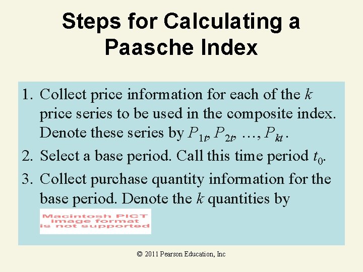
Steps for Calculating a Paasche Index 1. Collect price information for each of the k price series to be used in the composite index. Denote these series by P 1 t, P 2 t, …, Pkt. 2. Select a base period. Call this time period t 0. 3. Collect purchase quantity information for the base period. Denote the k quantities by © 2011 Pearson Education, Inc

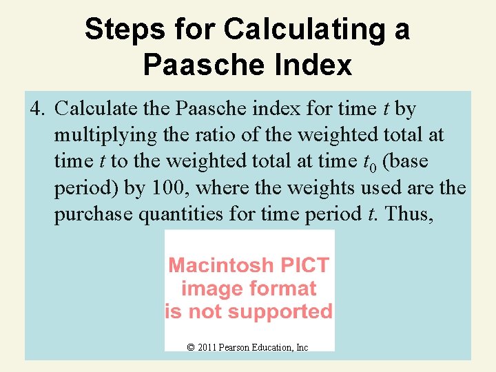
Steps for Calculating a Paasche Index 4. Calculate the Paasche index for time t by multiplying the ratio of the weighted total at time t to the weighted total at time t 0 (base period) by 100, where the weights used are the purchase quantities for time period t. Thus, © 2011 Pearson Education, Inc

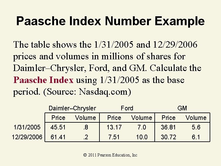
Paasche Index Number Example The table shows the 1/31/2005 and 12/29/2006 prices and volumes in millions of shares for Daimler–Chrysler, Ford, and GM. Calculate the Paasche Index using 1/31/2005 as the base period. (Source: Nasdaq. com) Daimler–Chrysler Ford GM Price Volume 1/31/2005 45. 51 . 8 13. 17 7. 0 36. 81 5. 6 12/29/2006 61. 41 . 2 7. 51 10. 0 30. 72 6. 1 © 2011 Pearson Education, Inc

Paasche Index Solution © 2011 Pearson Education, Inc

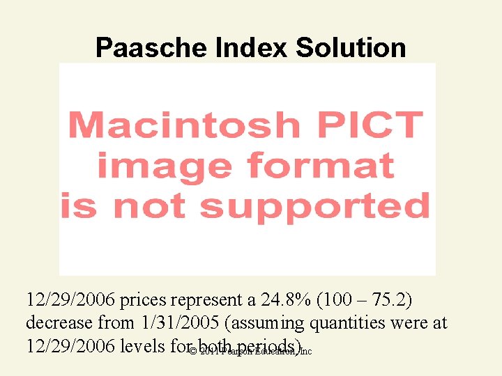
Paasche Index Solution 12/29/2006 prices represent a 24. 8% (100 – 75. 2) decrease from 1/31/2005 (assuming quantities were at 12/29/2006 levels for©both periods) 2011 Pearson Education, Inc

13. 2 Descriptive Analysis: Exponential Smoothing © 2011 Pearson Education, Inc

Exponential Smoothing • Type of weighted average • Removes rapid fluctuations in time series (less sensitive to short–term changes in prices) • Allows overall trend to be identified • Used forecasting future values • Exponential smoothing constant (w) affects “smoothness” of series © 2011 Pearson Education, Inc

Exponential Smoothing Constant Exponential smoothing constant, 0 < w < 1 • w close to 0 – More weight given to previous values of time series – Smoother series • w close to 1 – More weight given to current value of time series – Series looks similar to original (more variable) © 2011 Pearson Education, Inc

Steps for Calculating an Exponentially Smoothed Series 1. Select an exponential smoothing constant, w, between 0 and 1. Remember that small values of w give less weight to the current value of the series and yield a smoother series. Larger choices of w assign more weight to the current value of the series and yield a more variable series. © 2011 Pearson Education, Inc

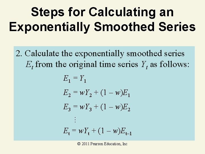
Steps for Calculating an Exponentially Smoothed Series 2. Calculate the exponentially smoothed series Et from the original time series Yt as follows: E 1 = Y 1 E 2 = w. Y 2 + (1 – w)E 1 … E 3 = w. Y 3 + (1 – w)E 2 Et = w. Yt + (1 – w)Et– 1 © 2011 Pearson Education, Inc

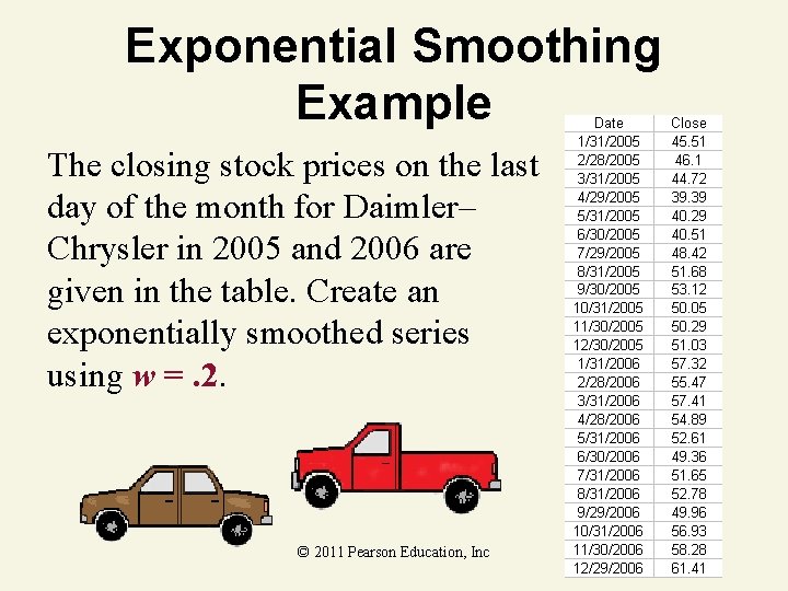
Exponential Smoothing Example The closing stock prices on the last day of the month for Daimler– Chrysler in 2005 and 2006 are given in the table. Create an exponentially smoothed series using w =. 2. © 2011 Pearson Education, Inc

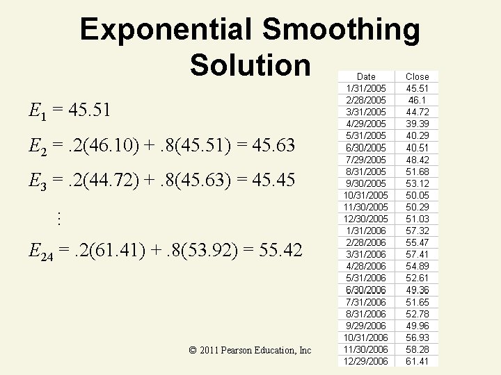
Exponential Smoothing Solution E 1 = 45. 51 E 2 =. 2(46. 10) +.

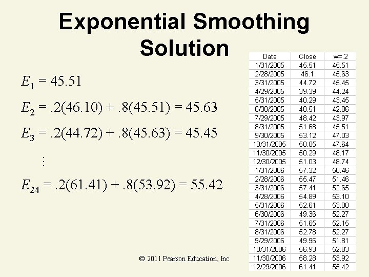
Exponential Smoothing Solution Actual Series Smoothed Series (w =. 2) © 2011 Pearson Education,

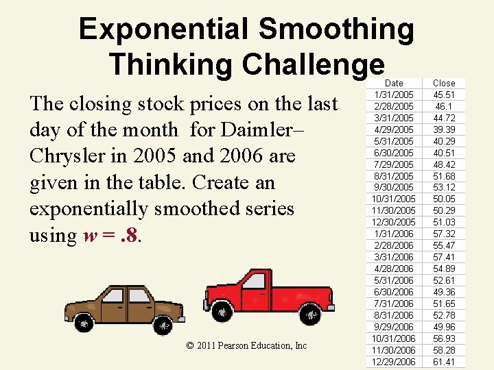
Exponential Smoothing Thinking Challenge The closing stock prices on the last day of the month for Daimler– Chrysler in 2005 and 2006 are given in the table. Create an exponentially smoothed series using w =. 8. © 2011 Pearson Education, Inc

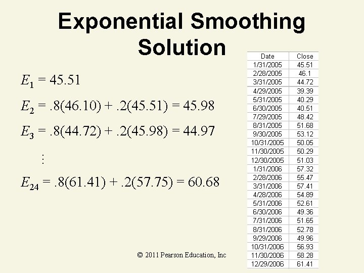
Exponential Smoothing Solution E 1 = 45. 51 E 2 =. 8(46. 10) +.

13. 3 Time Series Components © 2011 Pearson Education, Inc

Descriptive v. Inferential Analysis • Descriptive Analysis – Picture of the behavior of the time series – e. g. Index numbers, exponential smoothing – No measure of reliability • Inferential Analysis – Goal: Forecasting future values – Measure of reliability © 2011 Pearson Education, Inc

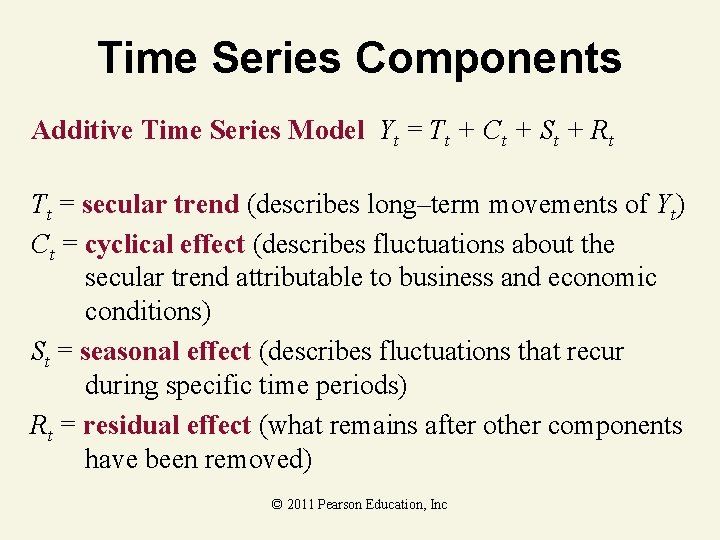
Time Series Components Additive Time Series Model Yt = Tt + Ct + St + Rt Tt = secular trend (describes long–term movements of Yt) Ct = cyclical effect (describes fluctuations about the secular trend attributable to business and economic conditions) St = seasonal effect (describes fluctuations that recur during specific time periods) Rt = residual effect (what remains after other components have been removed) © 2011 Pearson Education, Inc

13. 4 Forecasting: Exponential Smoothing © 2011 Pearson Education, Inc

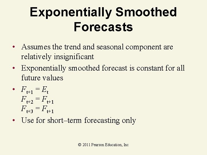
Exponentially Smoothed Forecasts • Assumes the trend and seasonal component are relatively insignificant • Exponentially smoothed forecast is constant for all future values • Ft+1 = Et Ft+2 = Ft+1 Ft+3 = Ft+1 • Use for short–term forecasting only © 2011 Pearson Education, Inc

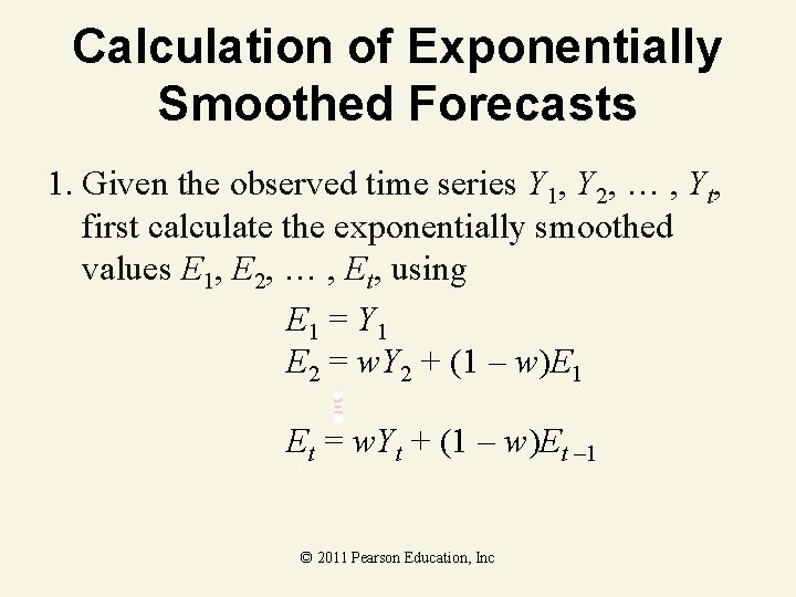
Calculation of Exponentially Smoothed Forecasts 1. Given the observed time series Y 1, Y 2, … , Yt, first calculate the exponentially smoothed values E 1, E 2, … , Et, using E 1 = Y 1 E 2 = w. Y 2 + (1 – w)E 1 Et = w. Yt + (1 – w)Et – 1 © 2011 Pearson Education, Inc

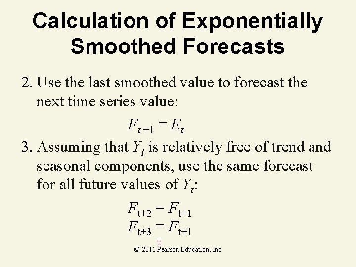
Calculation of Exponentially Smoothed Forecasts 2. Use the last smoothed value to forecast the next time series value: Ft +1 = Et 3. Assuming that Yt is relatively free of trend and seasonal components, use the same forecast for all future values of Yt: Ft+2 = Ft+1 Ft+3 = Ft+1 © 2011 Pearson Education, Inc

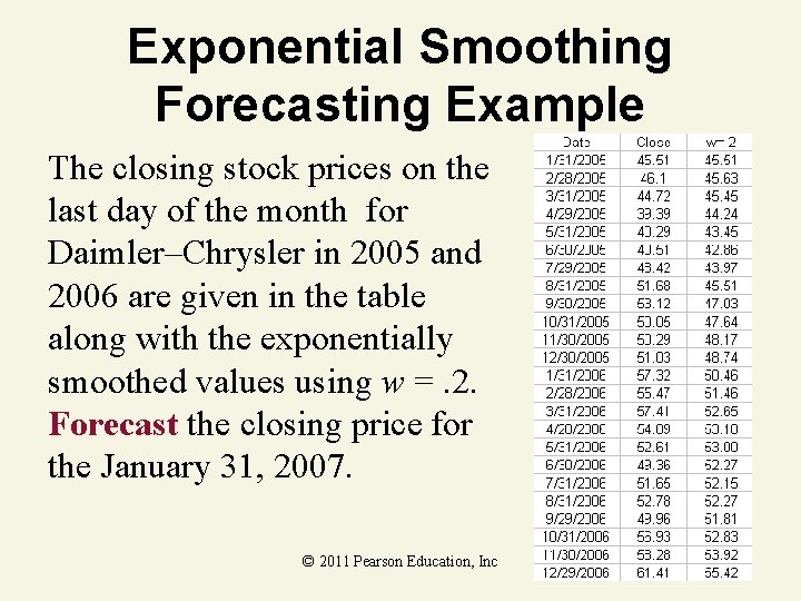
Exponential Smoothing Forecasting Example The closing stock prices on the last day of the month for Daimler–Chrysler in 2005 and 2006 are given in the table along with the exponentially smoothed values using w =. 2. Forecast the closing price for the January 31, 2007. © 2011 Pearson Education, Inc

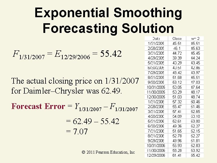
Exponential Smoothing Forecasting Solution F 1/31/2007 = E 12/29/2006 = 55. 42 The actual closing price on 1/31/2007 for Daimler–Chrysler was 62. 49. Forecast Error = Y 1/31/2007 – F 1/31/2007 = 62. 49 – 55. 42 = 7. 07 © 2011 Pearson Education, Inc

13. 5 Forecasting Trends: Holt’s Method © 2011 Pearson Education, Inc

The Holt Forecasting Model • Accounts for trends in time series • Two components – Exponentially smoothed component, Et • Smoothing constant 0 < w < 1 – Trend component, Tt • Smoothing constant 0 < v < 1 – Close to 0: More weight to past trend – Close to 1: More weight to recent trend © 2011 Pearson Education, Inc

Steps for Calculating Components of the Holt Forecasting Model 1. Select an exponential smoothing constant w between 0 and 1. Small values of w give less weight to the current values of the time series and more weight to the past. Larger choices assign more weight to the current value of the series. © 2011 Pearson Education, Inc

Steps for Calculating Components of the Holt Forecasting Model 2. Select a trend smoothing constant v between 0 and 1. Small values of v give less weight to the current changes in the level of the series and more weight to the past trend. Larger values assign more weight to the most recent trend of the series and less to past trends. © 2011 Pearson Education, Inc

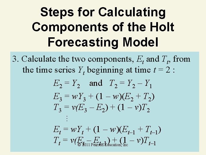
Steps for Calculating Components of the Holt Forecasting Model … 3. Calculate the two components, Et and Tt, from the time series Yt beginning at time t = 2 : E 2 = Y 2 and T 2 = Y 2 – Y 1 E 3 = w. Y 3 + (1 – w)(E 2 + T 2) T 3 = v(E 3 – E 2) + (1 – v)T 2 Et = w. Yt + (1 – w)(Et– 1 + Tt– 1) Tt = v(E Et– 1 Education, ) + (1 Inc – v)Tt– 1 t –Pearson © 2011

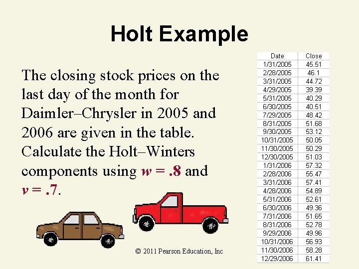
Holt Example The closing stock prices on the last day of the month for Daimler–Chrysler in 2005 and 2006 are given in the table. Calculate the Holt–Winters components using w =. 8 and v =. 7. © 2011 Pearson Education, Inc

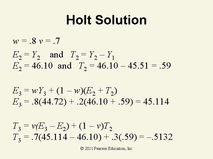
Holt Solution w =. 8 v =. 7 E 2 = Y 2 and T 2 = Y 2 – Y 1 E 2 = 46. 10 and T 2 = 46. 10 – 45. 51 =. 59 E 3 = w. Y 3 + (1 – w)(E 2 + T 2) E 3 =. 8(44. 72) +. 2(46. 10 +. 59) = 45. 114 T 3 = v(E 3 – E 2) + (1 – v)T 2 T 3 =. 7(45. 114 – 46. 10) +. 3(. 59) = –. 5132 © 2011 Pearson Education, Inc

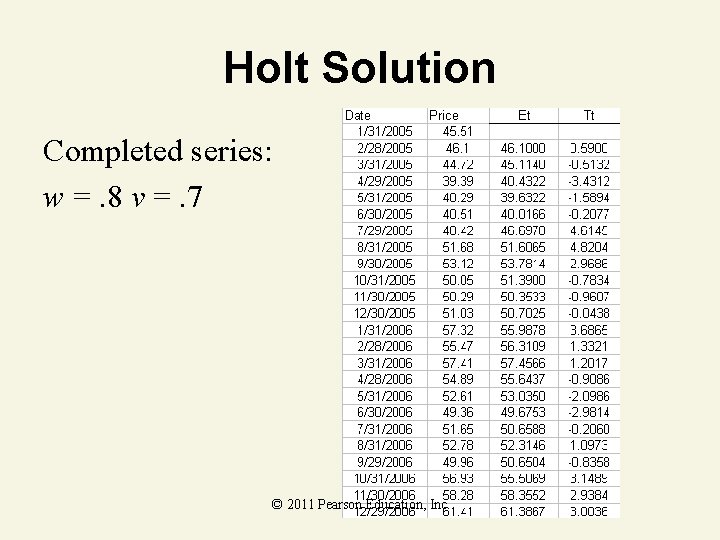
Holt Solution Completed series: w =. 8 v =. 7 © 2011 Pearson Education,

Holt Solution Holt exponentially smoothed (w =. 8 and v =. 7) Smoothed Actual

Holt’s Forecasting Methodology 1. Calculate the exponentially smoothed and trend components, Et and Tt, for each observed value of Yt (t ≥ 2) using the formulas given in the previous box. 2. Calculate the one-step-ahead forecast using Ft+1 = Et + Tt 3. Calculate the k-step-ahead forecast using Ft+k = Et + k. Tt © 2011 Pearson Education, Inc

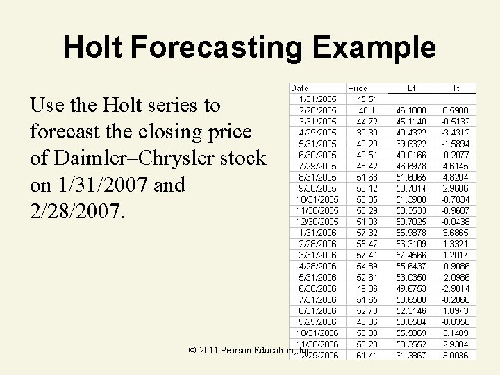
Holt Forecasting Example Use the Holt series to forecast the closing price of Daimler–Chrysler

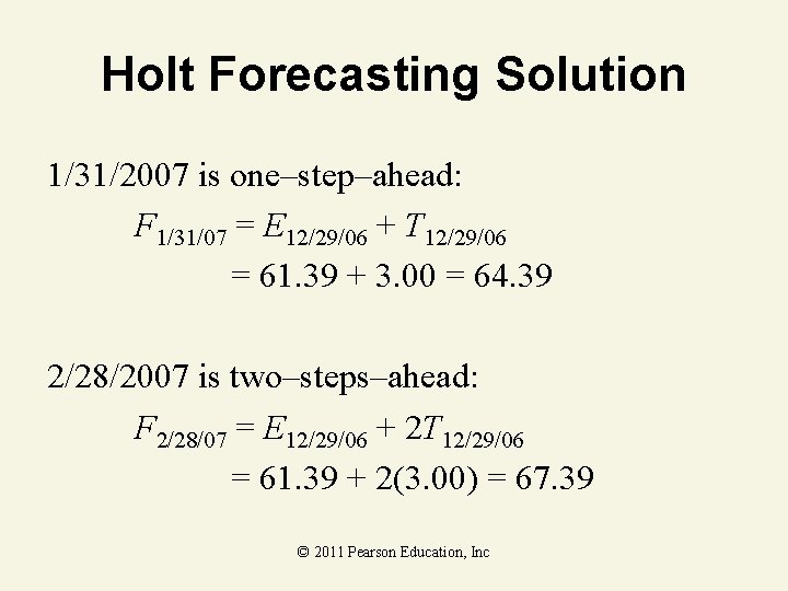
Holt Forecasting Solution 1/31/2007 is one–step–ahead: F 1/31/07 = E 12/29/06 + T 12/29/06 = 61. 39 + 3. 00 = 64. 39 2/28/2007 is two–steps–ahead: F 2/28/07 = E 12/29/06 + 2 T 12/29/06 = 61. 39 + 2(3. 00) = 67. 39 © 2011 Pearson Education, Inc

Holt Thinking Challenge The data shows the average undergraduate tuition at all 4–year institutions for the years 1996– 2004 (Source: U. S. Dept. of Education). Calculate the Holt– Winters components using w =. 7 and v =. 5. © 2011 Pearson Education, Inc

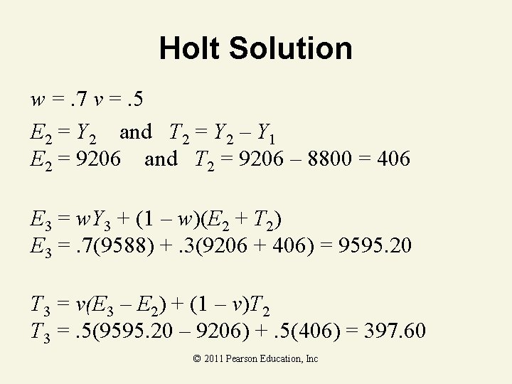
Holt Solution w =. 7 v =. 5 E 2 = Y 2 and T 2 = Y 2 – Y 1 E 2 = 9206 and T 2 = 9206 – 8800 = 406 E 3 = w. Y 3 + (1 – w)(E 2 + T 2) E 3 =. 7(9588) +. 3(9206 + 406) = 9595. 20 T 3 = v(E 3 – E 2) + (1 – v)T 2 T 3 =. 5(9595. 20 – 9206) +. 5(406) = 397. 60 © 2011 Pearson Education, Inc

Holt Solution Completed series © 2011 Pearson Education, Inc

Holt Solution Tuition Holt–Winters exponentially smoothed (w =. 7 and v =. 5) Actual

Holt Forecasting Thinking Challenge Use the Holt–Winters series to forecast tuition in 2005 and

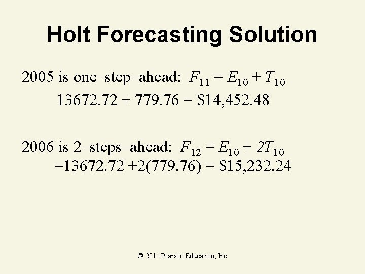
Holt Forecasting Solution 2005 is one–step–ahead: F 11 = E 10 + T 10 13672. 72 + 779. 76 = $14, 452. 48 2006 is 2–steps–ahead: F 12 = E 10 + 2 T 10 =13672. 72 +2(779. 76) = $15, 232. 24 © 2011 Pearson Education, Inc

13. 6 Measuring Forecast Accuracy: MAD and RMSE © 2011 Pearson Education, Inc

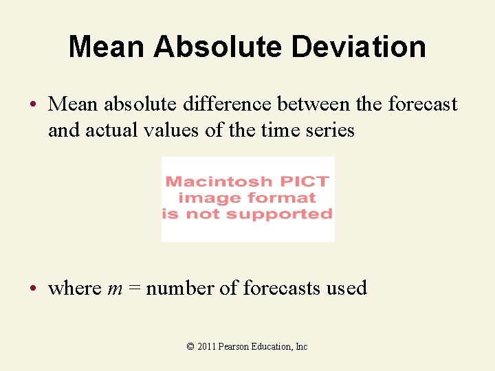
Mean Absolute Deviation • Mean absolute difference between the forecast and actual values of

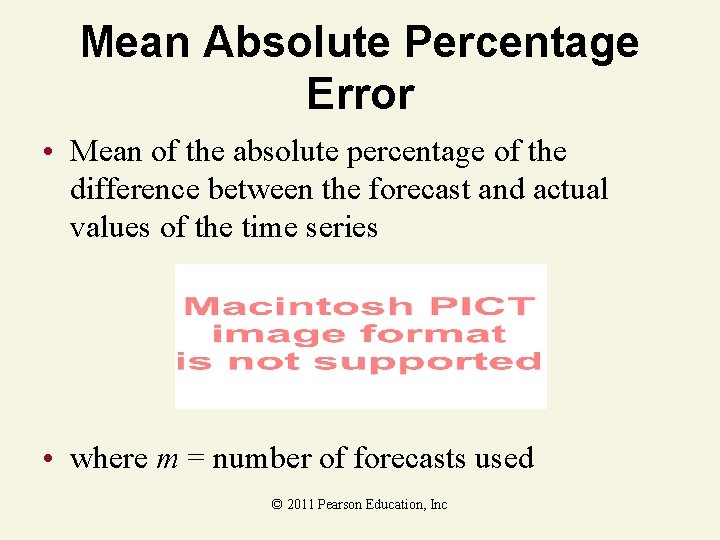
Mean Absolute Percentage Error • Mean of the absolute percentage of the difference between the forecast and actual values of the time series • where m = number of forecasts used © 2011 Pearson Education, Inc

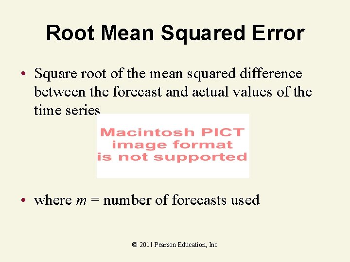
Root Mean Squared Error • Square root of the mean squared difference between the

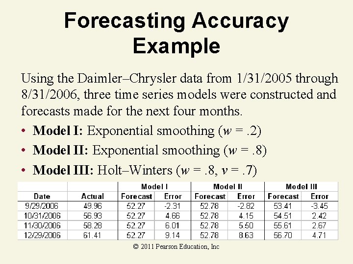
Forecasting Accuracy Example Using the Daimler–Chrysler data from 1/31/2005 through 8/31/2006, three time series models were constructed and forecasts made for the next four months. • Model I: Exponential smoothing (w =. 2) • Model II: Exponential smoothing (w =. 8) • Model III: Holt–Winters (w =. 8, v =. 7) © 2011 Pearson Education, Inc

Forecasting Accuracy Example Model I © 2011 Pearson Education, Inc

Forecasting Accuracy Example Model II © 2011 Pearson Education, Inc

Forecasting Accuracy Example Model III © 2011 Pearson Education, Inc

13. 7 Forecasting Trends: Simple Linear Regression © 2011 Pearson Education, Inc

Simple Linear Regression • Model: E(Yt) = β 0 + β 1 t • Relates time series, Yt, to time, t • Cautions – Risky to extrapolate (forecast beyond observed data) – Does not account for cyclical effects © 2011 Pearson Education, Inc

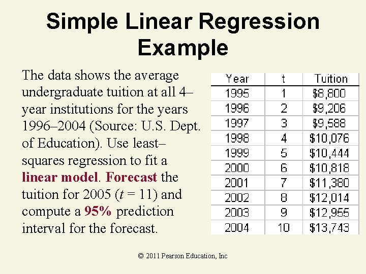
Simple Linear Regression Example The data shows the average undergraduate tuition at all 4– year institutions for the years 1996– 2004 (Source: U. S. Dept. of Education). Use least– squares regression to fit a linear model. Forecast the tuition for 2005 (t = 11) and compute a 95% prediction interval for the forecast. © 2011 Pearson Education, Inc

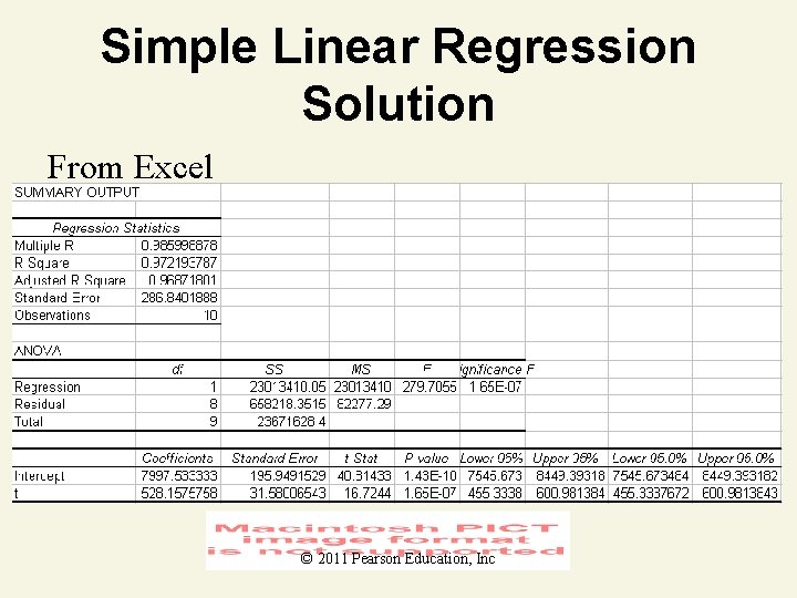
Simple Linear Regression Solution From Excel © 2011 Pearson Education, Inc

Simple Linear Regression Solution © 2011 Pearson Education, Inc

Simple Linear Regression Solution Forecast tuition for 2005 (t = 11): 95% prediction interval:

13. 8 Seasonal Regression Models © 2011 Pearson Education, Inc

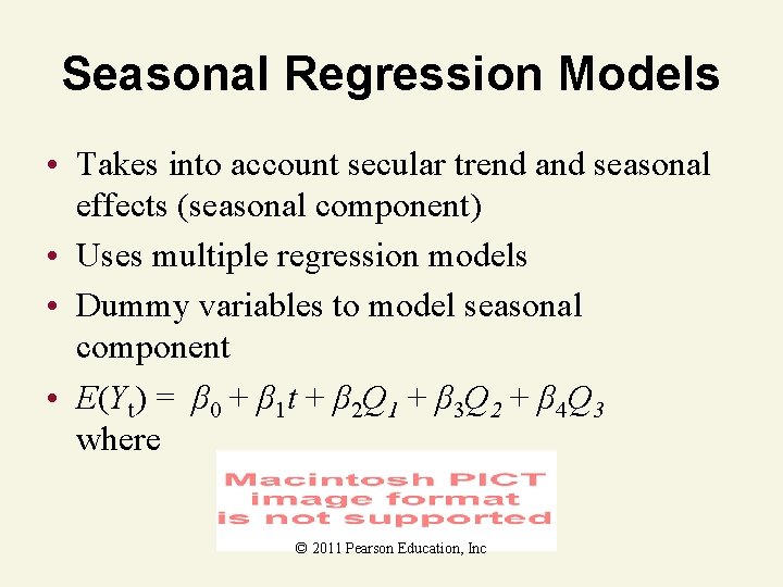
Seasonal Regression Models • Takes into account secular trend and seasonal effects (seasonal component) • Uses multiple regression models • Dummy variables to model seasonal component • E(Yt) = β 0 + β 1 t + β 2 Q 1 + β 3 Q 2 + β 4 Q 3 where © 2011 Pearson Education, Inc

13. 9 Autocorrelation and the Durbin-Watson Test © 2011 Pearson Education, Inc

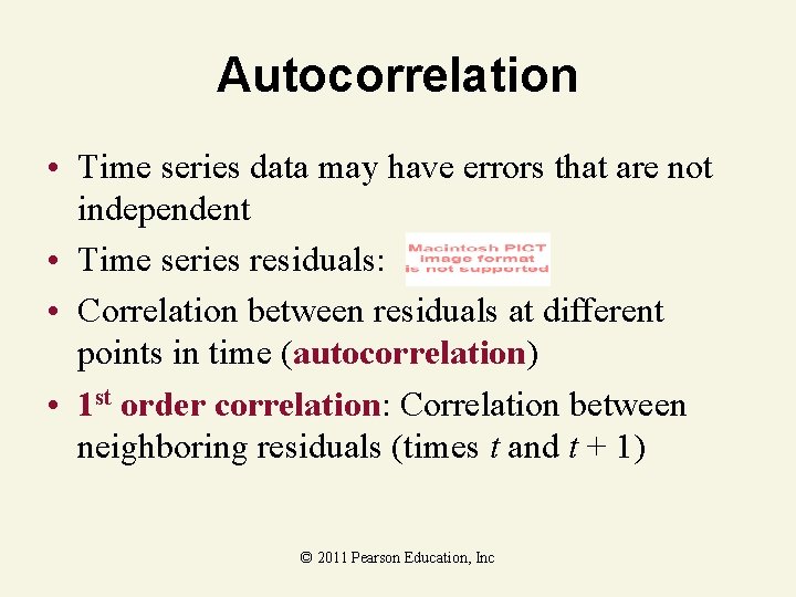
Autocorrelation • Time series data may have errors that are not independent • Time series residuals: • Correlation between residuals at different points in time (autocorrelation) • 1 st order correlation: Correlation between neighboring residuals (times t and t + 1) © 2011 Pearson Education, Inc

Autocorrelation Plot of residuals v. time for tuition data shows residuals tend to group

Durbin–Watson Test • H 0: No first–order autocorrelation of residuals • Ha: Positive first–order

Interpretation of Durbin. Watson d-Statistic 1. If the residuals are uncorrelated, then d ≈ 2. 2. If the residuals are positively autocorrelated, then d < 2, and if the autocorrelation is very strong, d ≈ 2. 3. If the residuals are negatively autocorrelated, then d >2, and if the autocorrelation is very strong, d ≈ 4. © 2011 Pearson Education, Inc

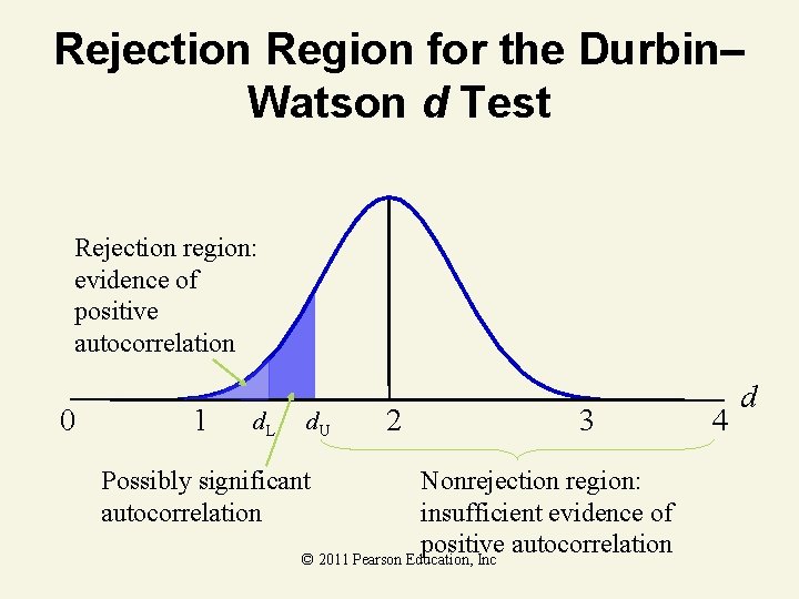
Rejection Region for the Durbin– Watson d Test Rejection region: evidence of positive autocorrelation 0 1 d. L d. U Possibly significant autocorrelation 2 3 Nonrejection region: insufficient evidence of positive autocorrelation © 2011 Pearson Education, Inc 4 d

Durbin–Watson d-Test for Autocorrelation One-tailed Test H 0: No first–order autocorrelation of residuals Ha: Positive first–order autocorrelation of residuals (or Ha: Negative first–order autocorrelation) Test Statistic © 2011 Pearson Education, Inc

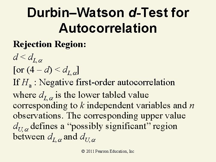
Durbin–Watson d-Test for Autocorrelation Rejection Region: d < d. L, [or (4 – d) < d. L, If Ha : Negative first-order autocorrelation where d. L, is the lower tabled value corresponding to k independent variables and n observations. The corresponding upper value d. U, defines a “possibly significant” region between d. L, and d. U, © 2011 Pearson Education, Inc

Durbin–Watson d-Test for Autocorrelation Two-tailed Test H 0: No first–order autocorrelation of residuals Ha: Positive or Negative first–order autocorrelation of residuals Test Statistic © 2011 Pearson Education, Inc

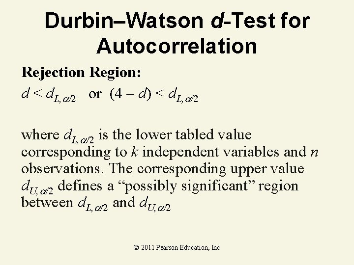
Durbin–Watson d-Test for Autocorrelation Rejection Region: d < d. L, or (4 – d) < d. L, where d. L, is the lower tabled value corresponding to k independent variables and n observations. The corresponding upper value d. U, defines a “possibly significant” region between d. L, and d. U, © 2011 Pearson Education, Inc

Requirements for the Validity of the d-Test The residuals are normally distributed. © 2011

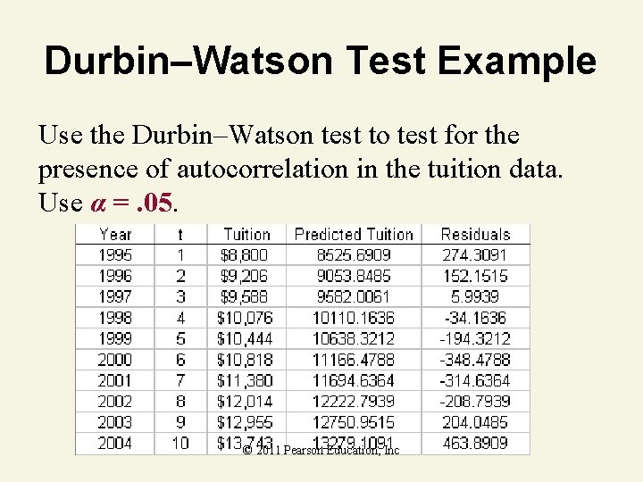
Durbin–Watson Test Example Use the Durbin–Watson test to test for the presence of autocorrelation

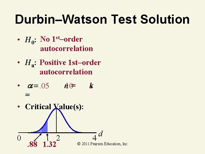
Durbin–Watson Test Solution • H 0: No 1 st–order autocorrelation • Ha: Positive 1

Durbin–Watson Solution Test Statistic © 2011 Pearson Education, Inc

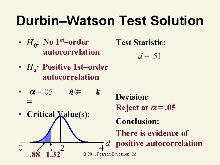
Durbin–Watson Test Solution • H 0: No 1 st–order autocorrelation Test Statistic: d =. 51 • Ha: Positive 1 st–order autocorrelation • n. 05 10= 1 k = • Critical Value(s): 0 2. 88 1. 32 4 Decision: Reject at =. 05 Conclusion: There is evidence of d positive autocorrelation © 2011 Pearson Education, Inc

Key Ideas Time Series Data generated by processes over time. © 2011 Pearson Education,

Key Ideas Index Number Measures the change in a variable over time relative to a base period. Types of Index numbers: 1. Simple index number 2. Simple composite index number 3. Weighted composite number (Laspeyers index or Pasche index) © 2011 Pearson Education, Inc

Key Ideas Time Series Components 1. 2. 3. 4. Secular (long-term) trend Cyclical effect

Key Ideas Time Series Forecasting Descriptive methods of forecasting with smoothing: 1. Exponential smoothing

Key Ideas Time Series Forecasting An Inferential forecasting method: least squares regression © 2011

Key Ideas Time Series Forecasting Measures of forecast accuracy: 1. mean absolute deviation (MAD) 2. mean absolute percentage error (MAPE) 3. root mean squared error (RMSE) © 2011 Pearson Education, Inc

Key Ideas Time Series Forecasting Problems with least squares regression forecasting: 1. Prediction outside the experimental region 2. Regression errors are autocorrelated © 2011 Pearson Education, Inc