2011 Pearson Education Inc Statistics for Business and

Statistics for Business and Economics Chapter 8 Design of Experiments and Analysis of Variance

Contents 8. 1 Elements of a Designed Experiment 8. 2 The Completely Randomized Design: Single Factor 8. 3 Multiple Comparisons of Means 8. 4 The Randomized Block Design 8. 5 Factorial Experiments: Two Factors © 2011 Pearson Education, Inc

Learning Objectives 1. Discuss critical elements in the design of a sampling experiment 2. Learn how to set up three experimental designs for comparing more than two population means: completely randomized, randomized block, and factorial design 3. Show to analyze data collected from a designed experiment using a technique called an analysis of variance (ANOVA) © 2011 Pearson Education, Inc

8. 1 Elements of a Designed Experiment © 2011 Pearson Education, Inc

Response Variable The response variable is the variable of interest to be measured in

Factors are those variables whose effect on the response is of interest to the experimenter. Quantitative factors are measured on a numerical scale, whereas qualitative factors are those that are not (naturally) measured on a numerical scale. Factors are also referred to as independent variables. © 2011 Pearson Education, Inc

Factor Levels Factor levels are the values of the factor used in the experiment.

Designed and Observational Experiment A designed experiment is one for which the analyst controls the specification of the treatments and the method of assigning the experimental units to each treatment. An observational experiment is one for which the analyst simply observes the treatments and the response on a sample of experimental units. © 2011 Pearson Education, Inc

Experimental Unit An experimental unit is the object on which the response and factors

Experiment • Investigator controls one or more independent variables – Called treatment variables or factors – Contain two or more levels (subcategories) • Observes effect on dependent variable – Response to levels of independent variable • Experimental design: plan used to test hypotheses © 2011 Pearson Education, Inc

Examples of Experiments 1. Thirty stores are randomly assigned 1 of 4 (levels) store displays (independent variable) to see the effect on sales (dependent variable). 2. Two hundred consumers are randomly assigned 1 of 3 (levels) brands of juice (independent variable) to study reaction (dependent variable). © 2011 Pearson Education, Inc

8. 2 The Completely Randomized Design: Single Factor © 2011 Pearson Education, Inc

Completely Randomized Design A completely randomized design is a design for which independent random

Completely Randomized Design • Experimental units (subjects) are assigned randomly to treatments – Subjects are assumed homogeneous • One factor or independent variable – Two or more treatment levels or classifications • Analyzed by one-way ANOVA © 2011 Pearson Education, Inc

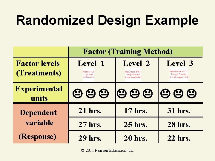
Randomized Design Example Factor (Training Method) Factor levels (Treatments) Experimental units Level 1 Level 2 Level 3 Dependent variable 21 hrs. 17 hrs. 31 hrs. 27 hrs. 25 hrs. 28 hrs. (Response) 29 hrs. 20 hrs. 22 hrs. © 2011 Pearson Education, Inc

ANOVA F-Test • • Tests the equality of two or more (k) population means Variables – One nominal scaled independent variable § Two or more (k) treatment levels or classifications – One interval or ratio scaled dependent variable • Used to analyze completely randomized experimental designs © 2011 Pearson Education, Inc

ANOVA F-Test to Compare k Treatment Means: Completely Randomized Design H 0: µ 1 = µ 2 = … = µk Ha: At least two treatment means differ Rejection region: F > F , where F is based on (k – 1) numerator degrees of freedom (associated with MST) and (n – k) denominator degrees of freedom (associated with MSE). © 2011 Pearson Education, Inc

Conditions Required for a Valid ANOVA F-test: Completely Randomized Design 1. The samples are randomly selected in an independent manner from the k treatment populations. (This can be accomplished by randomly assigning the experimental units to the treatments. ) 2. All k sampled populations have distributions that are approximately normal. 3. The k population variances are equal (i. e. , © 2011 Pearson Education, Inc

ANOVA F-Test Hypotheses • H 0: 1 = 2 = 3 =. . . = k — All population means are equal — No treatment effect f(x) • Ha: Not All i Are Equal — At least 2 pop. means are different — Treatment effect — 1 2 . . . k is Wrong 1 = 2 = 3 x f(x) © 2011 Pearson Education, Inc 1 = 2 3 x

Why Variances? • Same treatment variation Different treatment variation • Different random variation Same random variation A Pop 1 Pop 2 Pop 3 Pop 4 Pop 5 Pop 6 Variances WITHIN differ B Pop 1 Pop 4 Pop 2 Pop 3 Pop 5 Pop 6 Variances AMONG differ 2011 conclude Pearson Education, Inc Possible© to means are equal!

ANOVA Basic Idea 1. Compares two types of variation to test equality of means 2. Comparison basis is ratio of variances 3. If treatment variation is significantly greater than random variation then means are not equal 4. Variation measures are obtained by ‘partitioning’ total variation © 2011 Pearson Education, Inc

What Do You Do When the Assumptions Are Not Satisfied for an ANOVA for a Completely Randomized Design? Answer: Use a nonparametric statistical method such as the Kruskal-Wallis H-test. © 2011 Pearson Education, Inc

Steps for Conducting an ANOVA for a Completely Randomized Design 1. Be sure the design is truly completely randomized, with independent random samples for each treatment. 2. Check the assumptions of normality and equal variances. © 2011 Pearson Education, Inc

Steps for Conducting an ANOVA for a Completely Randomized Design 3. Create an ANOVA summary table that specifies the variability attributable to treatments and error, making sure that it leads to the calculation of the F-statistic for testing the null hypothesis that the treatment means are equal in the population. Use a statistical software program to obtain the numerical results. If no such package is available, use the calculation formulas in Appendix C. © 2011 Pearson Education, Inc

Steps for Conducting an ANOVA for a Completely Randomized Design 4. If the F-test leads to the conclusion that the means differ, a. Conduct a multiple comparisons procedure for as many of the pairs of means as you wish to compare. Use the results to summarize the statistically significant differences among the treatment means. b. If desired, form confidence intervals for one or more individual treatment means. © 2011 Pearson Education, Inc

Steps for Conducting an ANOVA for a Completely Randomized Design 5. If the F-test leads to the nonrejection of the null hypothesis that the treatment means are equal, consider the following possibilities: a. The treatment means are equal–that is, the null hypothesis is true. © 2011 Pearson Education, Inc

Steps for Conducting an ANOVA for a Completely Randomized Design b. The treatment means really differ, but other important factors affecting the response are not accounted for by the completely randomized design. These factors inflate the sampling variability, as measured by MSE, resulting in smaller values of the F-statistic. Either increase the sample size for each treatment or use a different experimental design that accounts for the other factors affecting the response. © 2011 Pearson Education, Inc

Steps for Conducting an ANOVA for a Completely Randomized Design Note: Be careful not to automatically conclude that the treatment means are equal because the possibility of a Type II error must be considered if you accept H 0. © 2011 Pearson Education, Inc

ANOVA Partitions Total Variation Total variation Variation due to treatment • • Variation due to random sampling Sum of Squares Among Sum of Squares Between Sum of Squares Treatment Among Groups Variation • Sum of Squares Within • Sum of Squares Error • Within Groups Variation © 2011 Pearson Education, Inc

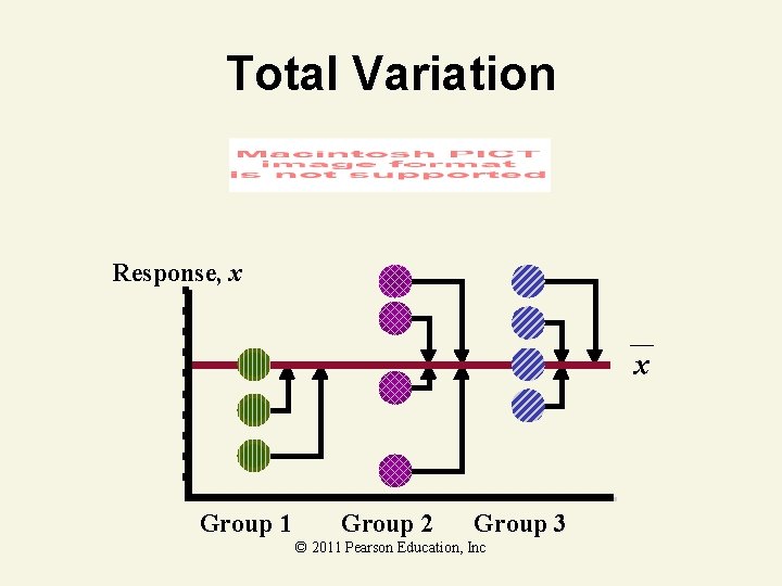
Total Variation Response, x x Group 1 Group 2 Group 3 © 2011 Pearson

Treatment Variation Response, x x 3 x 2 x 1 Group 2 Group 3

Random (Error) Variation Response, x x 3 x 2 x 1 Group 2 Group

ANOVA F-Test Statistic 1. Test Statistic • F = MST / MSE — MST is Mean Square for Treatment — MSE is Mean Square for Error 2. Degrees of Freedom • 1 = k – 1 numerator degrees of freedom 1. 2 = n – k denominator degrees of freedom — k = Number of groups 1. n = Total sample size © 2011 Pearson Education, Inc

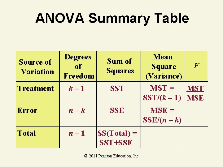
ANOVA Summary Table Source of Variation Degrees of Freedom Treatment k– 1 SST Error n–k SSE Total n– 1 SS(Total) = SST+SSE Sum of Squares © 2011 Pearson Education, Inc Mean F Square (Variance) MST = MST SST/(k – 1) MSE = SSE/(n – k)

ANOVA F-Test Critical Value If means are equal, F = MST / MSE 1. Only reject large F! Reject H 0 Do Not Reject H 0 0 F(α; k – 1, n – k) Always One-Tail! © 1984 -1994 T/Maker Co. © 2011 Pearson Education, Inc F

ANOVA F-Test Example As production manager, you Mach 1 Mach 2 Mach 3 want to see if three filling machines have different mean 25. 40 23. 40 20. 00 26. 31 21. 80 22. 20 filling times. You assign 15 24. 10 23. 50 19. 75 similarly trained and experienced workers, 5 per 23. 74 22. 75 20. 60 machine, to the machines. At 25. 10 21. 60 20. 40 the. 05 level of significance, is there a difference in mean filling times? © 2011 Pearson Education, Inc

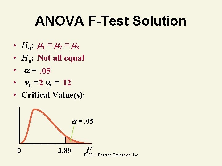
ANOVA F-Test Solution H 0: 1 = 2 = 3 Ha: Not all equal

Summary Table Solution From Computer Source of Variation Degrees of Freedom Mean Sum of Squares (Variance) Treatment (Machines) 3– 1=2 47. 1640 23. 5820 Error 15 – 3 = 12 11. 0532 . 9211 Total 15 – 1 = 14 58. 2172 © 2011 Pearson Education, Inc F 25. 60

ANOVA F-Test Solution H 0: 1 = 2 = 3 Ha: Not all equal =. 05 1 = 2 2 = 12 Critical Value(s): • • • =. 05 0 3. 89 Test Statistic: F MST MSE 23. 5820. 9211 25. 6 Decision: Reject at =. 05 Conclusion: There is evidence population F © 2011 Pearsonmeans Education, Incare different

ANOVA F-Test Thinking Challenge You’re a trainer for Microsoft Corp. Is there a difference in mean learning times of 12 people using 4 different training methods ( =. 05)? M 1 M 2 M 3 M 4 10 11 13 18 9 16 8 23 5 9 9 25 Use the following table. © 2011 Pearson Education, Inc © 1984 -1994 T/Maker Co.

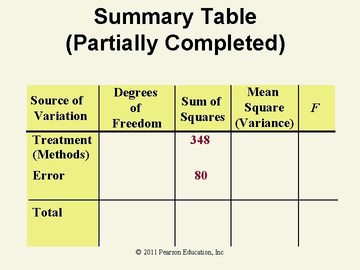
Summary Table (Partially Completed) Source of Variation Treatment (Methods) Error Degrees of Freedom Mean

ANOVA F-Test Solution H 0: 1 = 2 = 3 = 4 Ha: Not

Summary Table Solution Source of Variation Degrees of Freedom Mean Sum of Squares (Variance) Treatment (Methods) 4– 1=3 348 116 Error 12 – 4 = 8 80 10 Total 12 – 1 = 11 428 © 2011 Pearson Education, Inc F 11. 6

ANOVA F-Test Solution H 0: 1 = 2 = 3 = 4 Ha: Not all equal =. 05 1 = 3 2 = 8 Critical Value(s): • • • =. 05 0 4. 07 Test Statistic: F MST MSE 116 10 11. 6 Decision: Reject at =. 05 Conclusion: There is evidence population F means are different © 2011 Pearson Education, Inc

8. 3 Multiple Comparisons of Means © 2011 Pearson Education, Inc

Determining the Number of Pairwise Comparisons of Treatment Means In general, if there are

Tukey Methods Tukey methods. For each of these procedures, the risk of making a Type I error applies to the comparisons of the treatment means in the experiment; thus, the value of selected is called an experimentwise error rate (in contrast to a comparisonwise error rate). © 2011 Pearson Education, Inc

Bonferroni Method The Bonferroni method (see Miller, 1981), like the Tukey procedure, can be applied when pairwise comparisons are of interest; however, Bonferroni’s method does not require equal sample sizes. © 2011 Pearson Education, Inc

Scheffé Method Scheffé (1953) developed a more general procedure for comparing all possible linear combinations of treatment means (called contrasts). Consequently, when making pairwise comparisons, the confidence intervals produced by Scheffé’s method will generally be wider than the Tukey or Bonferroni confidence intervals. © 2011 Pearson Education, Inc

Tukey Procedure • Tells which population means are significantly different – Example: μ 1 = μ 2 ≠ μ 3 f(x) • Post hoc procedure – Done after rejection of equal means in ANOVA • Output from many statistical computer programs © 2011 Pearson Education, Inc 1 = 2 3 2 Groupings x

Guidelines © 2011 Pearson Education, Inc

8. 4 The Randomized Block Design © 2011 Pearson Education, Inc

Randomized Block Design The randomized block design consists of a twostep procedure: 1. Matched sets of experimental units, called blocks, are formed, each block consisting of k experimental units (where k is the number of treatments). The b blocks should consist of experimental units that are as similar as possible. 2. One experimental unit from each block is randomly assigned to each treatment, resulting in a total of n = bk responses. © 2011 Pearson Education, Inc

Randomized Block Design • • • Reduces sampling variability (MSE) Matched sets of experimental units (blocks) One experimental unit from each block is randomly assigned to each treatment © 2011 Pearson Education, Inc

Randomized Block Design Total Variation Partitioning © 2011 Pearson Education, Inc

ANOVA F-Test to Compare k Treatment Means: Randomized Block Design H 0: µ 1 = µ 2 = … = µk Ha: At least two treatment means differ Rejection region: F > F , where F is based on (k – 1) numerator degrees of freedom and (n – b – k +1) denominator degrees of freedom. © 2011 Pearson Education, Inc

Conditions Required for a Valid ANOVA F-test: Randomized Block Design 1. The b blocks are randomly selected, and all k treatments are applied (in random order) to each block. 2. The distributions of observations corresponding to all bk block-treatment combinations are approximately normal. 3. All bk block-treatment distributions have equal variances. © 2011 Pearson Education, Inc

Randomized Block Design F-Test Statistic 1. Test Statistic • F = MST / MSE — — MST is Mean Square for Treatment MSE is Mean Square for Error 2. Degrees of Freedom • 1 = k – 1 (numerator) 2 = n – k – b + 1 (denominator) — k = Number of groups 1. n = Total sample size 2. b = Number of blocks © 2011 Pearson Education, Inc

Randomized Block Design Example A production manager wants to see if three assembly methods have different mean assembly times (in minutes). Five employees were selected at random and assigned to use each assembly method. At the. 05 level of significance, is there a difference in mean assembly times? Employee Method 1 Method 2 Method 3 1 5. 4 3. 6 4. 0 2 4. 1 3. 8 2. 9 3 6. 1 5. 6 4. 3 4 3. 6 2. 3 2. 6 Education, Inc 5 5. 3 © 2011 Pearson 4. 7 3. 4

Random Block Design F-Test Solution H 0: 1 = 2 = 3 Ha: Not

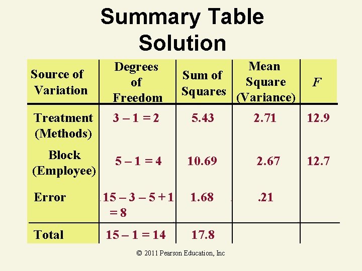
Summary Table Solution Source of Variation Degrees of Freedom Mean Sum of Squares (Variance) F Treatment (Methods) 3– 1=2 5. 43 2. 71 12. 9 Block (Employee) 5– 1=4 10. 69 2. 67 12. 7 Error 15 – 3 – 5 + 1 =8 1. 68 . 21 Total 15 – 1 = 14 17. 8 © 2011 Pearson Education, Inc

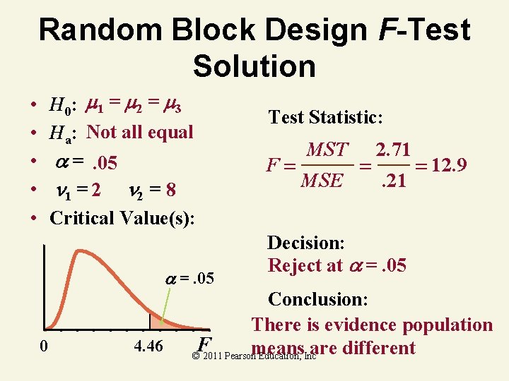
Random Block Design F-Test Solution H 0: 1 = 2 = 3 Ha: Not all equal =. 05 1 = 2 2 = 8 Critical Value(s): • • • =. 05 0 4. 46 Test Statistic: F MST MSE 2. 71. 21 12. 9 Decision: Reject at =. 05 Conclusion: There is evidence population F means are different © 2011 Pearson Education, Inc

Steps for Conducting an ANOVA for a Randomized Block Design 1. Be sure the design consists of blocks (preferably, blocks of homogeneous experimental units) and that each treatment is randomly assigned to one experimental unit in each block. 2. If possible, check the assumptions of normality and equal variances for all block-treatment combinations. [Note: This may be difficult to do because the design will likely have only one observation for each blocktreatment combination. ] © 2011 Pearson Education, Inc

Steps for Conducting an ANOVA for a Randomized Block Design 3. Create an ANOVA summary table that specifies the variability attributable to Treatments, Blocks, and Error, which leads to the calculation of the F-statistic to test the null hypothesis that the treatment means are equal in the population. Use a statistical software package or the calculation formulas in Appendix C to obtain the necessary numerical ingredients. © 2011 Pearson Education, Inc

Steps for Conducting an ANOVA for a Randomized Block Design 4. If the F-test leads to the conclusion that the means differ, use the Bonferroni, Tukey, or similar procedure to conduct multiple comparisons of as many of the pairs of means as you wish. Use the results to summarize the statistically significant differences among the treatment means. Remember that, in general, the randomized block design cannot be used to form confidence intervals for individual treatment means. © 2011 Pearson Education, Inc

Steps for Conducting an ANOVA for a Randomized Block Design 5. If the F-test leads to the nonrejection of the null hypothesis that the treatment means are equal, consider the following possibilities: a. The treatment means are equal–that is, the null hypothesis is true. © 2011 Pearson Education, Inc

Steps for Conducting an ANOVA for a Randomized Block Design b. The treatment means really differ, but other important factors affecting the response are not accounted for by the randomized block design. These factors inflate the sampling variability, as measured by MSE, resulting in smaller values of the F-statistic. Either increase the sample size for each treatment or conduct an experiment that accounts for the other factors affecting the response. Do not automatically reach the former conclusion because the possibility of a Type II error must be considered if you accept H 0. © 2011 Pearson Education, Inc

Steps for Conducting an ANOVA for a Randomized Block Design 6. If desired, conduct the F-test of the null hypothesis that the block means are equal. Rejection of this hypothesis lends statistical support to using the randomized block design. © 2011 Pearson Education, Inc

Steps for Conducting an ANOVA for a Randomized Block Design Note: It is often difficult to check whether the assumptions for a randomized block design are satisfied. There is usually one observation for each block-treatment combination. When you feel these assumptions are likely to be violated, a nonparametric procedure is advisable. © 2011 Pearson Education, Inc

What Do You Do When the Assumptions Are Not Satisfied for an ANOVA for a Completely Randomized Design? Answer: Use a nonparametric statistical method such as the Friedman Fr test. © 2011 Pearson Education, Inc

8. 5 Factorial Experiments: Two Factors © 2011 Pearson Education, Inc

Factorial Design A complete factorial experiment is one in which every factor-level combination is employed–that is, the number of treatments in the experiment equals the total number of factorlevel combinations. Also referred to as a two-way classification. © 2011 Pearson Education, Inc

Factorial Design To determine the nature of the treatment effect, if any, on the response in a factorial experiment, we need to break the treatment variability into three components: Interaction between Factors A and B, Main Effect of Factor A, and Main Effect of Factor B. The Factor Interaction component is used to test whether the factors combine to affect the response, while the Factor Main Effect components are used to determine whether the factors separately affect the response. © 2011 Pearson Education, Inc

Factorial Design • Experimental units (subjects) are assigned randomly to treatments – Subjects are assumed homogeneous • Two or more factors or independent variables – Each has two or more treatments (levels) • Analyzed by two-way ANOVA © 2011 Pearson Education, Inc

Procedure for Analysis of Two -Factorial Experiment 1. Partition the Total Sum of Squares into the Treatments and Error components. Use either a statistical software package or the calculation formulas in Appendix C to accomplish the partitioning. © 2011 Pearson Education, Inc

Procedure for Analysis of Two -Factorial Experiment 2. Use the F-ratio of Mean Square for Treatments to Mean Square for Error to test the null hypothesis that the treatment means are equal. a. If the test results in nonrejection of the null hypothesis, consider refining the experiment by increasing the number of replications or introducing other factors. Also consider the possibility that the response is unrelated to the two factors. b. If the test results in rejection of the null hypothesis, then proceed to step 3. © 2011 Pearson Education, Inc

Procedure for Analysis of Two -Factorial Experiment 3. Partition the Treatments Sum of Squares into the Main Effect and Interaction Sum of Squares. Use either a statistical software package or the calculation formulas in Appendix C to accomplish the partitioning. © 2011 Pearson Education, Inc

Procedure for Analysis of Two -Factorial Experiment 4. Test the null hypothesis that factors A and B do not interact to affect the response by computing the F-ratio of the Mean Square for Interaction to the Mean Square for Error. a. If the test results in nonrejection of the null hypothesis, proceed to step 5. b. If the test results in rejection of the null hypothesis, conclude that the two factors interact to affect the mean response. Then proceed to step 6 a. © 2011 Pearson Education, Inc

Procedure for Analysis of Two -Factorial Experiment 5. Conduct tests of two null hypotheses that the mean response is the same at each level of factor A and factor B. Compute two F-ratios by comparing the Mean Square for each Factor Main Effect to the Mean Square for Error. a. If one or both tests result in rejection of the null hypothesis, conclude that the factor affects the mean response. Proceed to step 6 b. © 2011 Pearson Education, Inc

Procedure for Analysis of Two -Factorial Experiment b. If both tests result in nonrejection, an apparent contradiction has occurred. Although the treatment means apparently differ (step 2 test), the interaction (step 4) and main effect (step 5) tests have not supported that result. Further experimentation is advised. © 2011 Pearson Education, Inc

Procedure for Analysis of Two -Factorial Experiment 6. Compare the means: a. If the test for interaction (step 4) is significant, use a multiple comparisons procedure to compare any or all pairs of the treatment means. b. If the test for one or both main effects (step 5) is significant, use a multiple comparisons procedure to compare the pairs of means corresponding to the levels of the significant factor(s). © 2011 Pearson Education, Inc

ANOVA Tests Conducted for Factorial Experiments: Completely Randomized Design, r Replicates per Treatment Test for Treatment Means H 0: No difference among the ab treatment means Ha: At least two treatment means differ Rejection region: F > F , based on (ab – 1) numerator and (n – ab) denominator degrees of freedom [Note: n = abr. ] © 2011 Pearson Education, Inc

ANOVA Tests Conducted for Factorial Experiments: Completely Randomized Design, r Replicates per Treatment Test for Factor Interaction H 0: Factors A and B do not interact to affect the response mean Ha: Factors A and B do interact to affect the response mean Rejection region: F > F , based on (a – 1)(b – 1) numerator and (n – ab) denominator degrees of © 2011 Pearson Education, Inc freedom

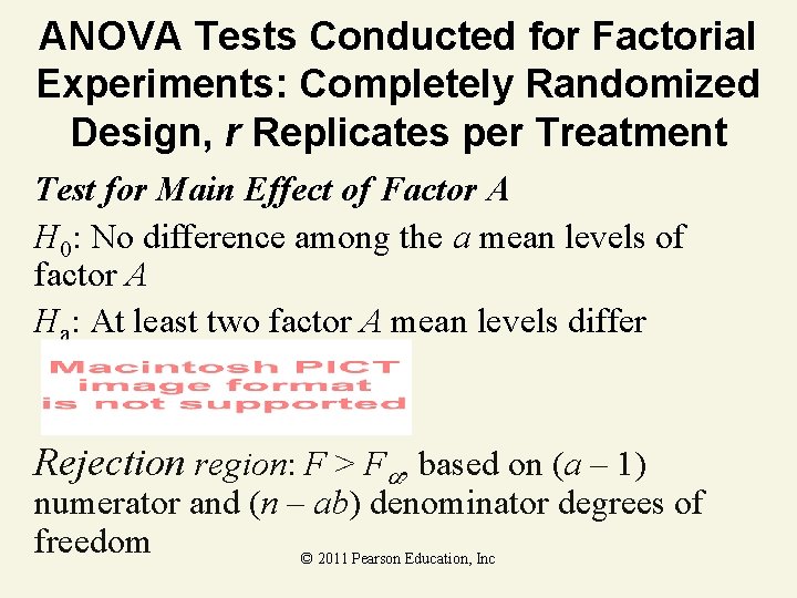
ANOVA Tests Conducted for Factorial Experiments: Completely Randomized Design, r Replicates per Treatment Test for Main Effect of Factor A H 0: No difference among the a mean levels of factor A Ha: At least two factor A mean levels differ Rejection region: F > F , based on (a – 1) numerator and (n – ab) denominator degrees of freedom © 2011 Pearson Education, Inc

ANOVA Tests Conducted for Factorial Experiments: Completely Randomized Design, r Replicates per Treatment Test for Main Effect of Factor B H 0: No difference among the b mean levels of factor B Ha: At least two factor B mean levels differ Rejection region: F > F , based on (b – 1) numerator and (n – ab) denominator degrees of freedom © 2011 Pearson Education, Inc

Conditions Required for Valid F-tests in Factorial Experiments 1. The response distribution for each factor-level combination (treatment) is normal. 2. The response variance is constant for all treatments. 3. Random and independent samples of experimental units are associated with each treatment. © 2011 Pearson Education, Inc

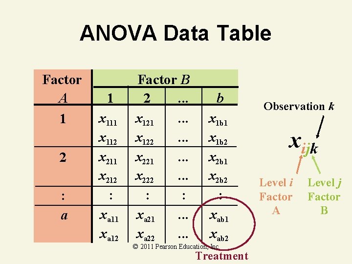
ANOVA Data Table Factor A 1 2 : a 1 x 112 x 211 x 212 : xa 11 xa 12 Factor B 2. . . x 121. . . x 122. . . x 221. . . x 222. . . : : xa 21. . . xa 22. . . b x 1 b 1 x 1 b 2 x 2 b 1 x 2 b 2 : xab 1 xab 2 © 2011 Pearson Education, Inc Treatment Observation k xijk Level i Factor A Level j Factor B

Factorial Design Example Factor Levels Factor 2 (Training Method) Level 1 Level 2 Level 3 11 hr. 27 hr. 29 hr. Level 1 15 hr. Factor 1 (High) (Motivation) Level 2 (Low) 12 hr. 15 hr. 17 hr. 10 hr. © 2011 Pearson Education, Inc 17 hr. 31 hr. 49 hr. 22 hr. Treatment

Advantages of Factorial Designs • Saves time and effort – e. g. , Could use separate completely randomized designs for each variable • Controls confounding effects by putting other variables into model • Can explore interaction between variables © 2011 Pearson Education, Inc

Two-Way ANOVA • Tests the equality of two or more population means when several independent variables are used • Same results as separate one-way ANOVA on each variable – No interaction can be tested • Used to analyze factorial designs © 2011 Pearson Education, Inc

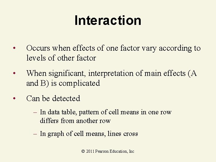
Interaction • Occurs when effects of one factor vary according to levels of other factor • When significant, interpretation of main effects (A and B) is complicated • Can be detected – In data table, pattern of cell means in one row differs from another row – In graph of cell means, lines cross © 2011 Pearson Education, Inc

Graphs of Interaction Effects of motivation (high or low) and training method (A, B, C) on mean learning time Interaction Average Response No Interaction High Average Response High Low A B C © 2011 Pearson Education, Inc Low A B C

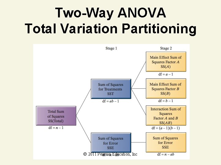
Two-Way ANOVA Total Variation Partitioning © 2011 Pearson Education, Inc

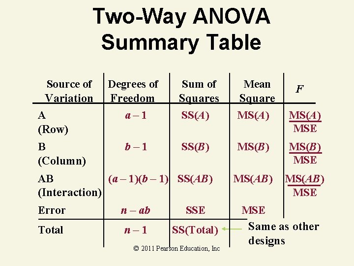
Two-Way ANOVA Summary Table Source of Variation A (Row) B (Column) Degrees of Freedom a– 1 b– 1 Sum of Squares SS(A) Mean Square MS(A) SS(B) MS(B) MSE MS(AB) MSE AB (a – 1)(b – 1) SS(AB) (Interaction) Error n – ab SSE Total n– 1 SS(Total) © 2011 Pearson Education, Inc F MS(A) MSE Same as other designs

Factorial Design Example Human Resources wants to determine if training time is different based on motivation level and training method. Conduct the appropriate ANOVA tests. Use α =. 05 for each test. Training Method Factor Levels Self– paced Classroom Computer 10 hr. 12 hr. Motivation 15 hr. 27 hr. Low 29 hr. Education, 17 Inchr. © 2011 Pearson High 15 hr. 11 hr. 22 hr. 17 hr. 31 hr. 49 hr.

Treatment Means F-Test Solution • H 0: The 6 treatment means are equal •

Two-Way ANOVA Summary Table Source of Variation Model Degrees of Freedom 5 Sum of Squares 1201. 8 Mean Square 240. 35 31. 42 Error 6 188. 5 Corrected Total 11 1390. 3 © 2011 Pearson Education, Inc F 7. 65

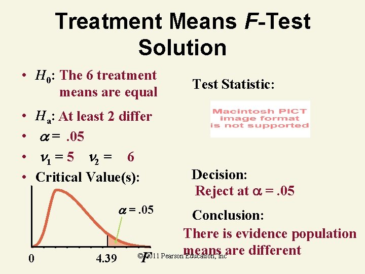
Treatment Means F-Test Solution • H 0: The 6 treatment means are equal • • Ha: At least 2 differ =. 05 1 = 5 2 = 6 Critical Value(s): =. 05 0 4. 39 Test Statistic: Decision: Reject at =. 05 Conclusion: There is evidence population © 2011 Pearsonmeans Education, Incare different F

Factor Interaction F-Test Solution • H 0: The factors do not interact • •

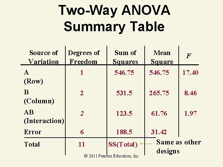
Two-Way ANOVA Summary Table Source of Variation A (Row) Degrees of Freedom Sum of Squares Mean Square 1 546. 75 17. 40 B (Column) 2 531. 5 265. 75 8. 46 AB (Interaction) 2 123. 5 61. 76 1. 97 Error 6 188. 5 Total 11 SS(Total) 31. 42 Same as other designs © 2011 Pearson Education, Inc F

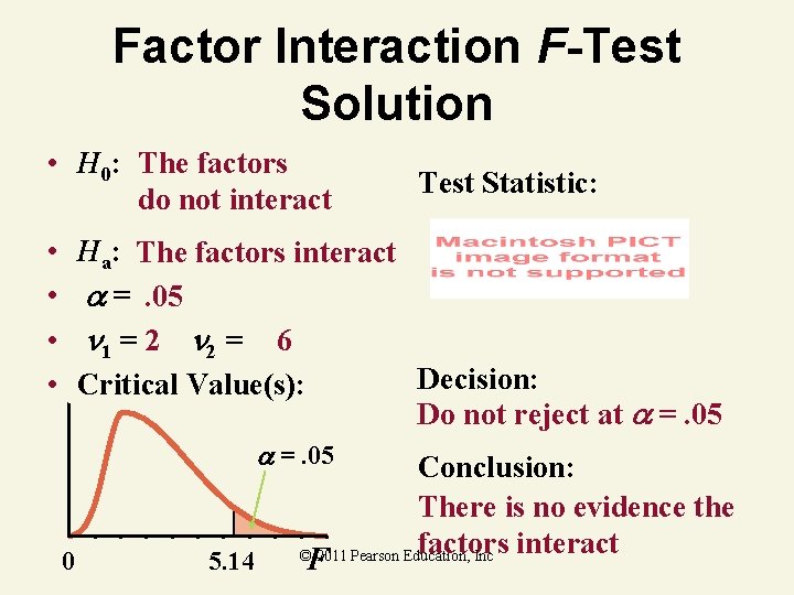
Factor Interaction F-Test Solution • H 0: The factors do not interact • • Test Statistic: Ha: The factors interact =. 05 1 = 2 2 = 6 Decision: Critical Value(s): Do not reject at =. 05 0 5. 14 Conclusion: There is no evidence the factors interact © 2011 Pearson Education, Inc F

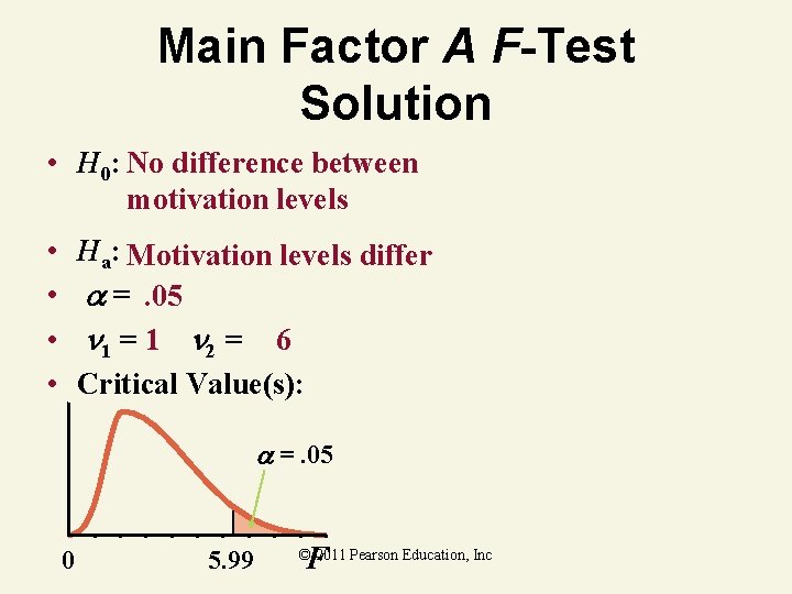
Main Factor A F-Test Solution • H 0: No difference between motivation levels •

Two-Way ANOVA Summary Table Source of Variation A (Row) Degrees of Freedom Sum of Squares Mean Square 1 546. 75 17. 40 B (Column) 2 531. 5 265. 75 8. 46 AB (Interaction) 2 123. 5 61. 76 1. 97 Error 6 188. 5 Total 11 SS(Total) 31. 42 Same as other designs © 2011 Pearson Education, Inc F

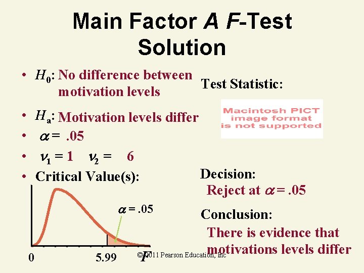
Main Factor A F-Test Solution • H 0: No difference between Test Statistic: motivation levels • • Ha: Motivation levels differ =. 05 1 = 1 2 = 6 Decision: Critical Value(s): Reject at =. 05 0 5. 99 Conclusion: There is evidence that motivations levels differ © 2011 Pearson Education, Inc F

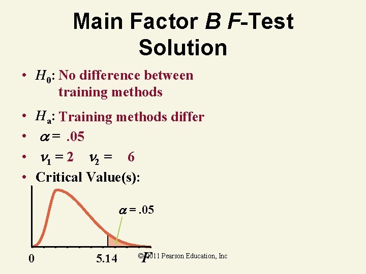
Main Factor B F-Test Solution • H 0: No difference between training methods •

Two-Way ANOVA Summary Table Source of Variation A (Row) Degrees of Freedom Sum of Squares Mean Square 1 546. 75 17. 40 B (Column) 2 531. 5 265. 75 8. 46 AB (Interaction) 2 123. 5 61. 76 1. 97 Error 6 188. 5 Total 11 SS(Total) 31. 42 Same as other designs © 2011 Pearson Education, Inc F

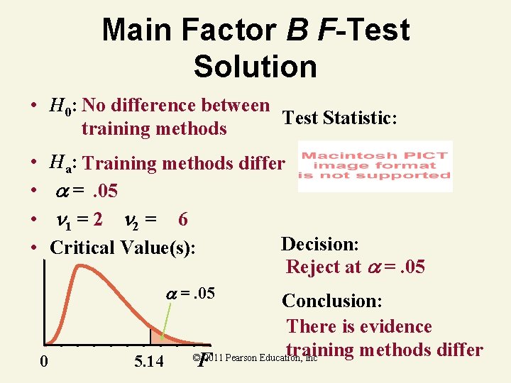
Main Factor B F-Test Solution • H 0: No difference between Test Statistic: training methods • • Ha: Training methods differ =. 05 1 = 2 2 = 6 Decision: Critical Value(s): Reject at =. 05 0 5. 14 Conclusion: There is evidence training methods differ © 2011 Pearson Education, Inc F

Key Ideas Key Elements of a Designed Experiment 1. Response (dependent) variable – quantitative 2. Factors (independent variables) – quantitative or qualitative 3. Factor levels (values of factors) – selected by the experimenter 4. Treatments – combinations of factor levels 5. Experimental units – assign treatments to experimental units and measure response for each © 2011 Pearson Education, Inc

Key Ideas Key Elements of a Designed Experiment Balanced Design Sample sizes for each treatment are equal. Test for main effects in a factorial design Only appropriate if the test for factor interaction is nonsignificant. Robust method Slight to moderate departures from normality do not have impact on validity of the ANOVA results. © 2011 Pearson Education, Inc

Key Ideas Conditions Required for Valid F-Test in a Completely Randomized Design 1. All

Key Ideas Conditions Required for Valid F-Test in a Randomized Block Design 1. All treatment-block populations are approximately normal. 2. All treatment-block populations have the same variance. © 2011 Pearson Education, Inc

Key Ideas Conditions Required for Valid F-Test in a Complete Factorial Design 1. All treatment populations are approximately normal. 2. All treatment populations have the same variance. Experimentwise error rate Risk of making at least one Type I error when making multiple comparisons of means in ANOVA © 2011 Pearson Education, Inc