2011 Pearson Education Inc Statistics for Business and
© 2011 Pearson Education, Inc
Statistics for Business and Economics Chapter 10 Simple Linear Regression © 2011 Pearson Education, Inc
Contents 10. 1 Probabilistic Models 10. 2 Fitting the Model: The Least Squares Approach 10. 3 Model Assumptions 10. 4 Assessing the Utility of the Model: Making Inferences about the Slope 1 © 2011 Pearson Education, Inc
Contents 10. 5 The Coefficients of Correlation and Determination 10. 6 Using the Model for Estimation and Prediction 10. 7 A Complete Example © 2011 Pearson Education, Inc
Learning Objectives • Introduce the straight-line (simple linear regression) model as a means of relating one quantitative variable to another quantitative variable • Introduce the correlation coefficient as a means of relating one quantitative variable to another quantitative variable © 2011 Pearson Education, Inc
Learning Objectives • Assess how well the simple linear regression model fits the sample data • Employ the simple linear regression model for predicting the value of one variable from a specified value of another variable © 2011 Pearson Education, Inc
10. 1 Probabilistic Models © 2011 Pearson Education, Inc
Models • • Representation of some phenomenon Mathematical model is a mathematical expression of some phenomenon Often describe relationships between variables Types – Deterministic models – Probabilistic models © 2011 Pearson Education, Inc
Deterministic Models • • • Hypothesize exact relationships Suitable when prediction error is negligible Example: force is exactly mass times acceleration – F = m·a © 2011 Pearson Education, Inc © 1984 -1994 T/Maker Co.
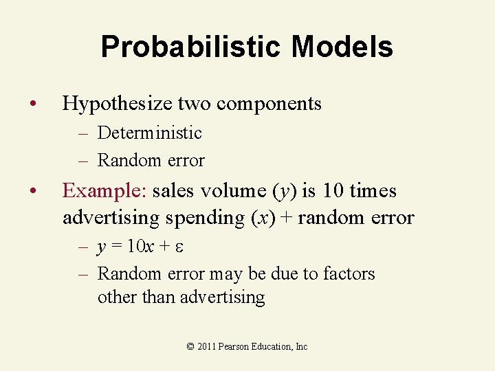
Probabilistic Models • Hypothesize two components – Deterministic – Random error • Example: sales volume (y) is 10 times advertising spending (x) + random error – y = 10 x + – Random error may be due to factors other than advertising © 2011 Pearson Education, Inc
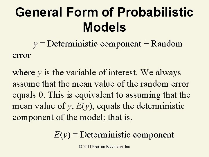
General Form of Probabilistic Models y = Deterministic component + Random error where y is the variable of interest. We always assume that the mean value of the random error equals 0. This is equivalent to assuming that the mean value of y, E(y), equals the deterministic component of the model; that is, E(y) = Deterministic component © 2011 Pearson Education, Inc
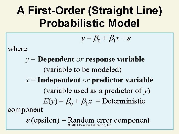
A First-Order (Straight Line) Probabilistic Model y = 0 + 1 x + where y = Dependent or response variable (variable to be modeled) x = Independent or predictor variable (variable used as a predictor of y) E(y) = 0 + 1 x = Deterministic component (epsilon) = ©Random error component 2011 Pearson Education, Inc
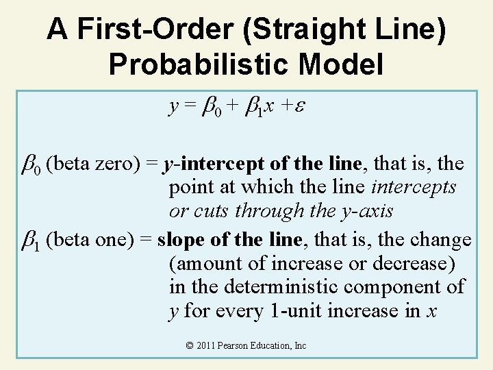
A First-Order (Straight Line) Probabilistic Model y = 0 + 1 x + 0 (beta zero) = y-intercept of the line, that is, the point at which the line intercepts or cuts through the y-axis 1 (beta one) = slope of the line, that is, the change (amount of increase or decrease) in the deterministic component of y for every 1 -unit increase in x © 2011 Pearson Education, Inc
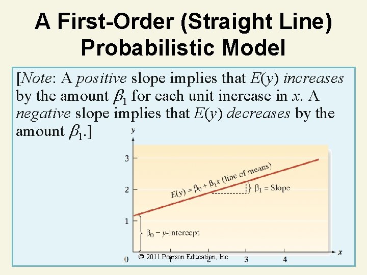
A First-Order (Straight Line) Probabilistic Model [Note: A positive slope implies that E(y) increases by the amount 1 for each unit increase in x. A negative slope implies that E(y) decreases by the amount 1. ] © 2011 Pearson Education, Inc
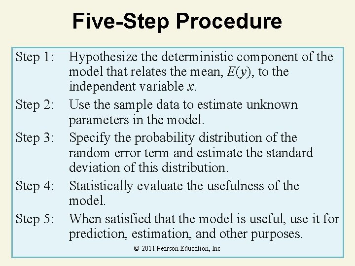
Five-Step Procedure Step 1: Step 2: Step 3: Step 4: Step 5: Hypothesize the deterministic component of the model that relates the mean, E(y), to the independent variable x. Use the sample data to estimate unknown parameters in the model. Specify the probability distribution of the random error term and estimate the standard deviation of this distribution. Statistically evaluate the usefulness of the model. When satisfied that the model is useful, use it for prediction, estimation, and other purposes. © 2011 Pearson Education, Inc
10. 2 Fitting the Model: The Least Squares Approach © 2011 Pearson Education, Inc
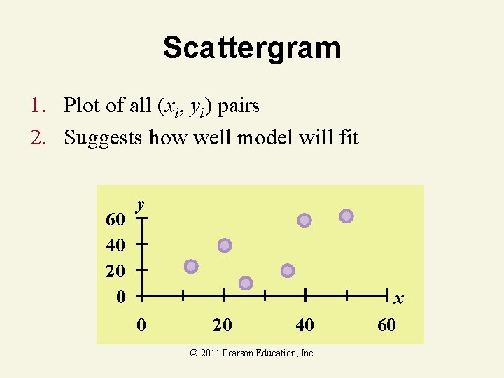
Scattergram 1. Plot of all (xi, yi) pairs 2. Suggests how well model will fit 60 40 20 0 y 0 20 40 © 2011 Pearson Education, Inc x 60
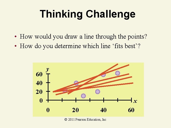
Thinking Challenge • How would you draw a line through the points? • How do you determine which line ‘fits best’? 60 40 20 0 y 0 20 40 © 2011 Pearson Education, Inc x 60
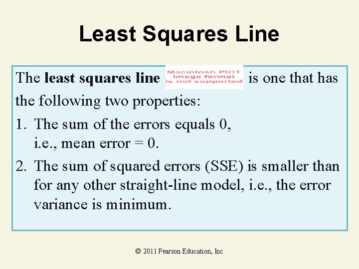
Least Squares Line The least squares line is one that has the following two properties: 1. The sum of the errors equals 0, i. e. , mean error = 0. 2. The sum of squared errors (SSE) is smaller than for any other straight-line model, i. e. , the error variance is minimum. © 2011 Pearson Education, Inc
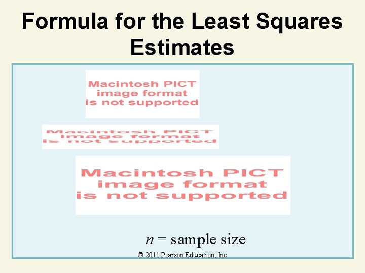
Formula for the Least Squares Estimates n = sample size © 2011 Pearson Education, Inc
Interpreting the Estimates of 0 and 1 in Simple Liner Regression y-intercept: represents the predicted value of y when x = 0 (Caution: This value will not be meaningful if the value x = 0 is nonsensical or outside the range of the sample data. ) slope: represents the increase (or decrease) in y for every 1 -unit increase in x (Caution: This interpretation is valid only for xvalues within the range of the sample data. ) © 2011 Pearson Education, Inc
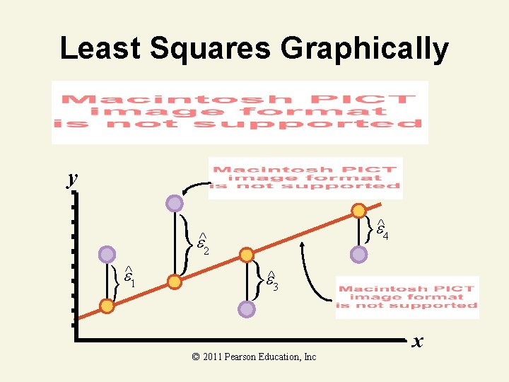
Least Squares Graphically y ^4 ^2 ^1 ^3 © 2011 Pearson Education, Inc x
Least Squares Example You’re a marketing analyst for Hasbro Toys. You gather the following data: Ad Expenditure (100$) Sales (Units) 1 1 2 1 3 2 4 2 5 4 Find the least squares line relating sales and advertising. © 2011 Pearson Education, Inc
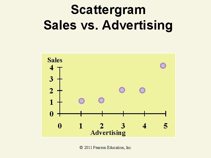
Scattergram Sales vs. Advertising Sales 4 3 2 1 0 0 1 2 3 Advertising © 2011 Pearson Education, Inc 4 5
Parameter Estimation Solution © 2011 Pearson Education, Inc
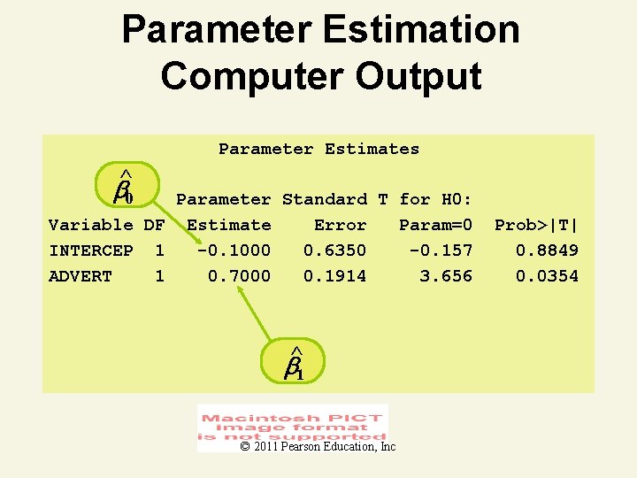
Parameter Estimation Computer Output Parameter Estimates ^0 Parameter Standard T for H 0: Variable DF Estimate Error Param=0 INTERCEP 1 -0. 1000 0. 6350 -0. 157 ADVERT 1 0. 7000 0. 1914 3. 656 ^1 © 2011 Pearson Education, Inc Prob>|T| 0. 8849 0. 0354
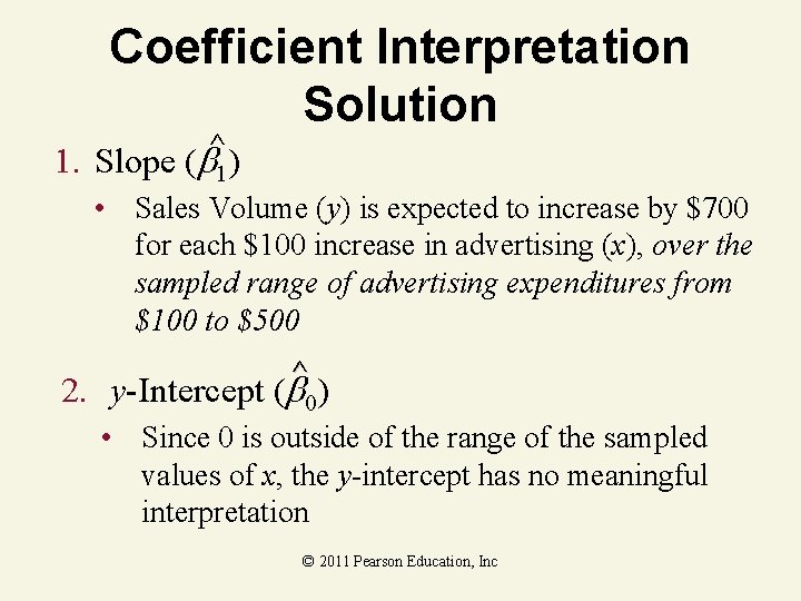
Coefficient Interpretation Solution ^ 1. Slope ( 1) • Sales Volume (y) is expected to increase by $700 for each $100 increase in advertising (x), over the sampled range of advertising expenditures from $100 to $500 ^ 2. y-Intercept ( 0) • Since 0 is outside of the range of the sampled values of x, the y-intercept has no meaningful interpretation © 2011 Pearson Education, Inc
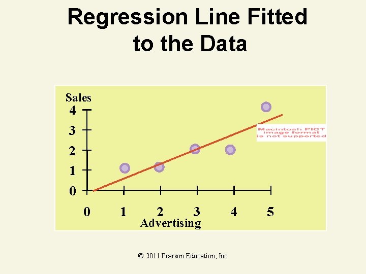
Regression Line Fitted to the Data Sales 4 3 2 1 0 0 1 2 3 Advertising © 2011 Pearson Education, Inc 4 5

Least Squares Thinking Challenge You’re an economist for the county cooperative. You gather the following data: Fertilizer (lb. ) Yield (lb. ) 4 3. 0 6 5. 5 10 6. 5 12 9. 0 Find the least squares line relating crop yield and fertilizer. © 1984 -1994 T/Maker Co. © 2011 Pearson Education, Inc
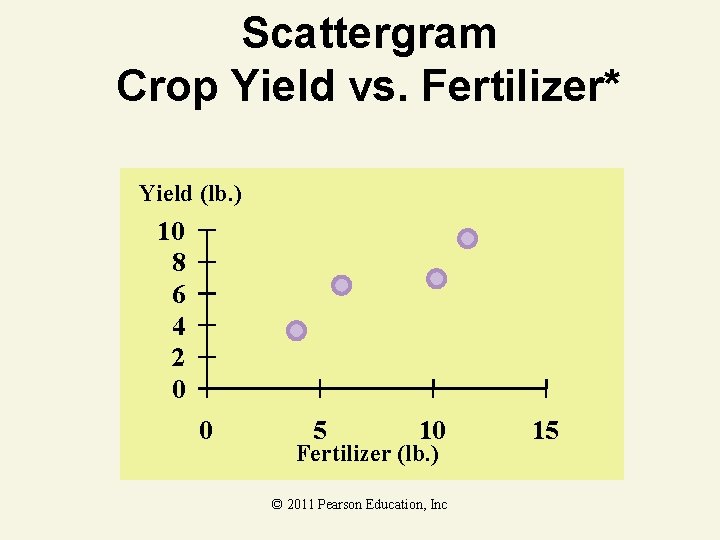
Scattergram Crop Yield vs. Fertilizer* Yield (lb. ) 10 8 6 4 2 0 0 5 10 Fertilizer (lb. ) © 2011 Pearson Education, Inc 15

Parameter Estimation Solution* © 2011 Pearson Education, Inc
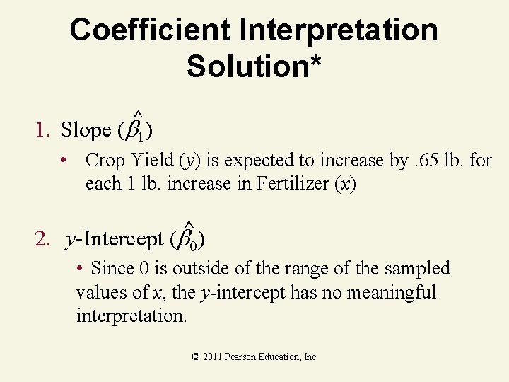
Coefficient Interpretation Solution* ^ 1. Slope ( 1) • Crop Yield (y) is expected to increase by. 65 lb. for each 1 lb. increase in Fertilizer (x) ^ 2. y-Intercept ( 0) • Since 0 is outside of the range of the sampled values of x, the y-intercept has no meaningful interpretation. © 2011 Pearson Education, Inc
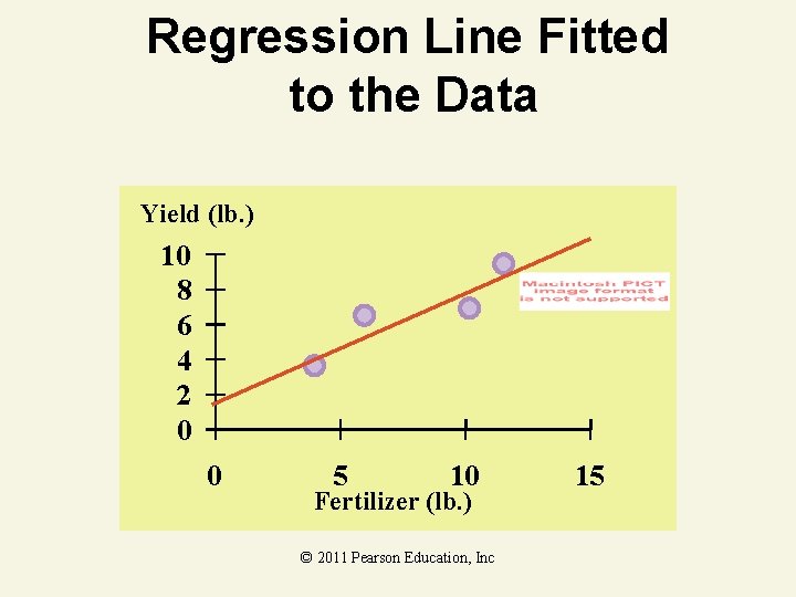
Regression Line Fitted to the Data Yield (lb. ) 10 8 6 4 2 0 0 5 10 Fertilizer (lb. ) © 2011 Pearson Education, Inc 15
10. 3 Model Assumptions © 2011 Pearson Education, Inc
Basic Assumptions of the Probability Distribution Assumption 1: The mean of the probability distribution of is 0 – that is, the average of the values of over an infinitely long series of experiments is 0 for each setting of the independent variable x. This assumption implies that the mean value of y, E(y), for a given value of x is E(y) = 0 + 1 x. © 2011 Pearson Education, Inc
Basic Assumptions of the Probability Distribution Assumption 2: The variance of the probability distribution of is constant for all settings of the independent variable x. For our straight-line model, this assumption means that the variance of is equal to a constant, say 2, for all values of x. © 2011 Pearson Education, Inc
Basic Assumptions of the Probability Distribution Assumption 3: The probability distribution of is normal. Assumption 4: The values of associated with any two observed values of y are independent–that is, the value of associated with one value of y has no effect on the values of associated with other y values. © 2011 Pearson Education, Inc
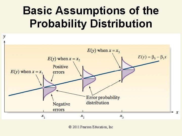
Basic Assumptions of the Probability Distribution. © 2011 Pearson Education, Inc
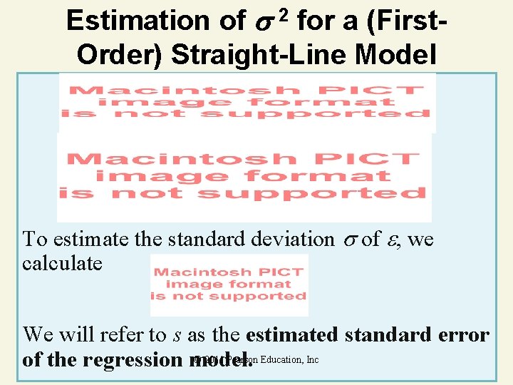
Estimation of 2 for a (First. Order) Straight-Line Model To estimate the standard deviation of , we calculate We will refer to s as the estimated standard error © 2011 Pearson Education, Inc of the regression model.
Calculating SSE, Example 2 s, s You’re a marketing analyst for Hasbro Toys. You gather the following data: Ad Expenditure (100$) Sales (Units) 1 1 2 1 3 2 4 2 5 4 Find SSE, s 2, and s. © 2011 Pearson Education, Inc
Calculating s 2 and s Solution © 2011 Pearson Education, Inc
10. 4 Assessing the Utility of the Model: Making Inferences about the Slope 1 © 2011 Pearson Education, Inc
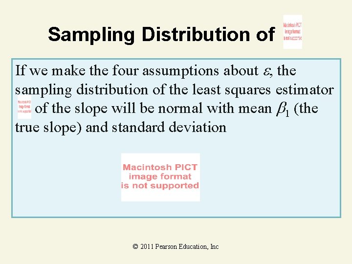
Sampling Distribution of If we make the four assumptions about , the sampling distribution of the least squares estimator of the slope will be normal with mean 1 (the true slope) and standard deviation © 2011 Pearson Education, Inc
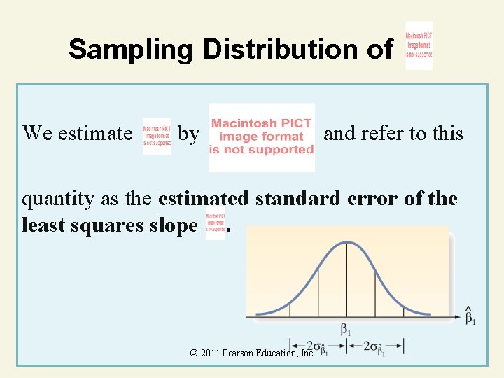
Sampling Distribution of We estimate by and refer to this quantity as the estimated standard error of the least squares slope. © 2011 Pearson Education, Inc
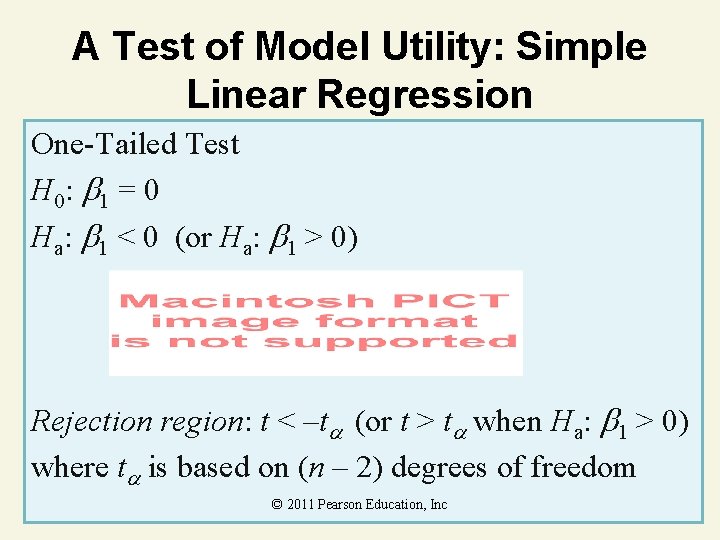
A Test of Model Utility: Simple Linear Regression One-Tailed Test H 0: 1 = 0 Ha: 1 < 0 (or Ha: 1 > 0) Rejection region: t < –t (or t > t when Ha: 1 > 0) where t is based on (n – 2) degrees of freedom © 2011 Pearson Education, Inc
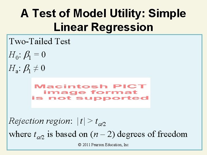
A Test of Model Utility: Simple Linear Regression Two-Tailed Test H 0: 1 = 0 Ha : 1 ≠ 0 Rejection region: | t | > t where t is based on (n – 2) degrees of freedom © 2011 Pearson Education, Inc
Interpreting p-Values for Coefficients in Regression Almost all statistical computer software packages report a two-tailed p-value for each of the parameters in the regression model. For example, in simple linear regression, the p-value for the twotailed test H 0: 1 = 0 versus Ha: 1 ≠ 0 is given on the printout. If you want to conduct a one-tailed test of hypothesis, you will need to adjust the p-value reported on the printout as follows: © 2011 Pearson Education, Inc
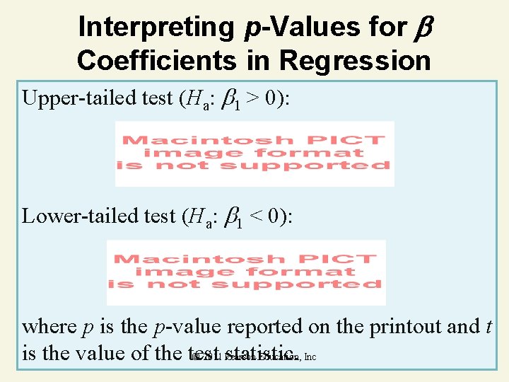
Interpreting p-Values for Coefficients in Regression Upper-tailed test (Ha: 1 > 0): Lower-tailed test (Ha: 1 < 0): where p is the p-value reported on the printout and t © 2011 Pearson Education, Inc is the value of the test statistic.
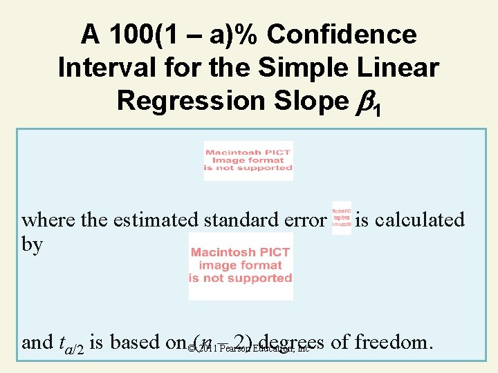
A 100(1 – a)% Confidence Interval for the Simple Linear Regression Slope 1 where the estimated standard error by is calculated and ta/2 is based on ©(n 2) Education, degrees of freedom. 2011– Pearson Inc
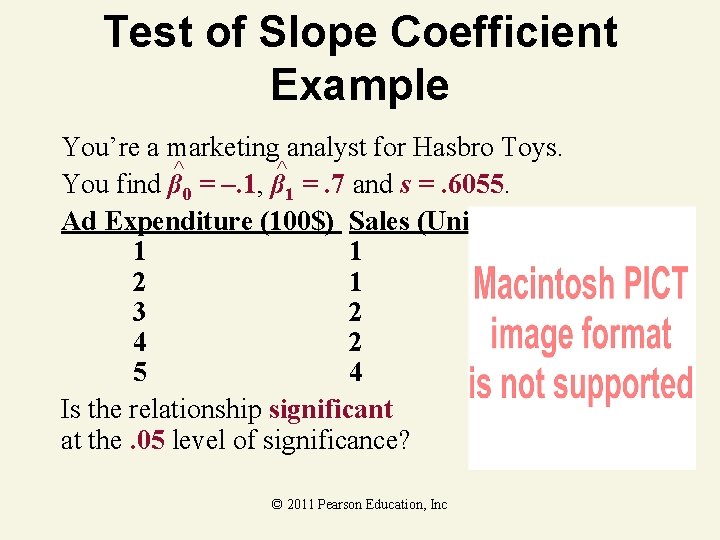
Test of Slope Coefficient Example You’re a marketing analyst for Hasbro Toys. ^ ^ You find β 0 = –. 1, β 1 =. 7 and s =. 6055. Ad Expenditure (100$) Sales (Units) 1 1 2 1 3 2 4 2 5 4 Is the relationship significant at the. 05 level of significance? © 2011 Pearson Education, Inc
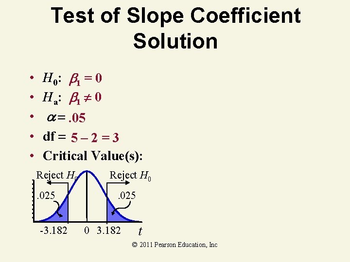
Test of Slope Coefficient Solution • • • H 0: 1 = 0 Ha: 1 0 . 05 df 5 – 2 = 3 Critical Value(s): Reject H 0. 025 -3. 182 Reject H 0. 025 0 3. 182 t © 2011 Pearson Education, Inc

Test Statistic Solution © 2011 Pearson Education, Inc
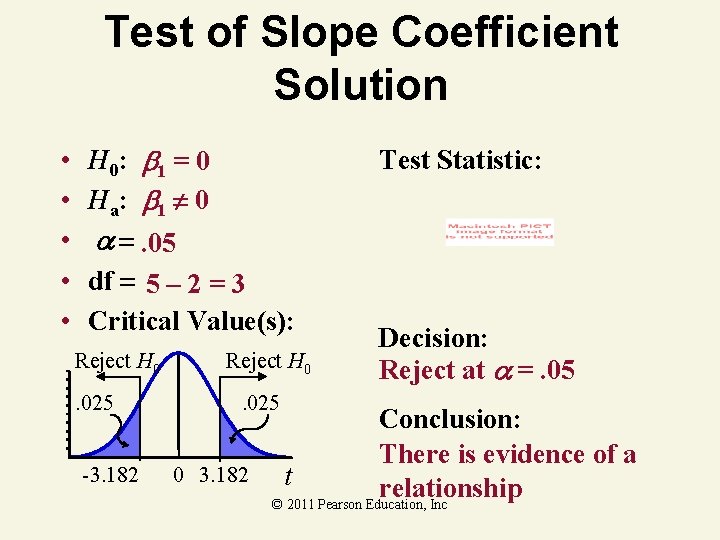
Test of Slope Coefficient Solution • • • H 0: 1 = 0 Ha: 1 0 . 05 df 5 – 2 = 3 Critical Value(s): Reject H 0. 025 -3. 182 Reject H 0. 025 0 3. 182 Test Statistic: Decision: Reject at =. 05 Conclusion: There is evidence of a t relationship © 2011 Pearson Education, Inc
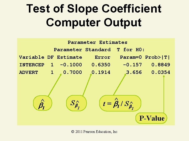
Test of Slope Coefficient Computer Output Parameter Estimates Parameter Standard T for H 0: Variable DF Estimate Error Param=0 Prob>|T| INTERCEP 1 -0. 1000 0. 6350 -0. 157 0. 8849 ADVERT 1 0. 7000 0. 1914 3. 656 0. 0354 ^ 1 S ^ 1 t = ^1 / S ^ 1 P-Value © 2011 Pearson Education, Inc
10. 5 The Coefficients of Correlation and Determination © 2011 Pearson Education, Inc
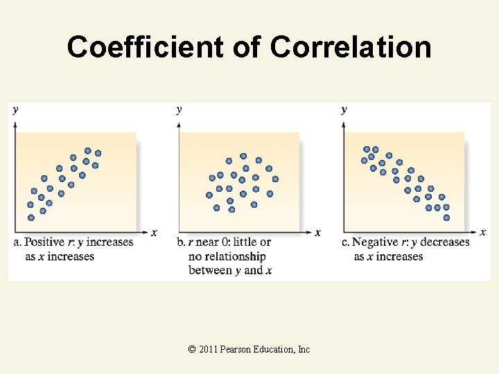
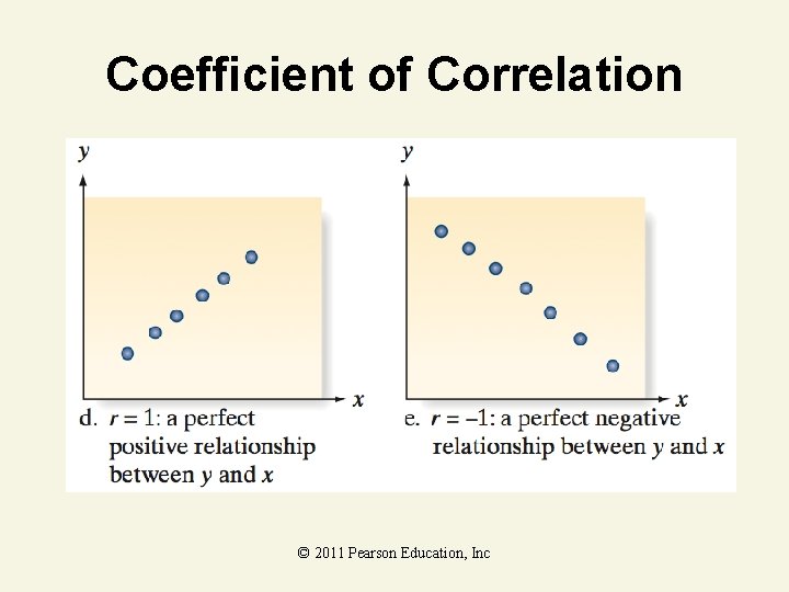
Correlation Models • • Answers ‘How strong is the linear relationship between two variables? ’ Coefficient of correlation – – Sample correlation coefficient denoted r Values range from – 1 to +1 Measures degree of association Does not indicate cause–effect relationship © 2011 Pearson Education, Inc
Coefficient of Correlation where © 2011 Pearson Education, Inc
Coefficient of Correlation © 2011 Pearson Education, Inc
Coefficient of Correlation © 2011 Pearson Education, Inc
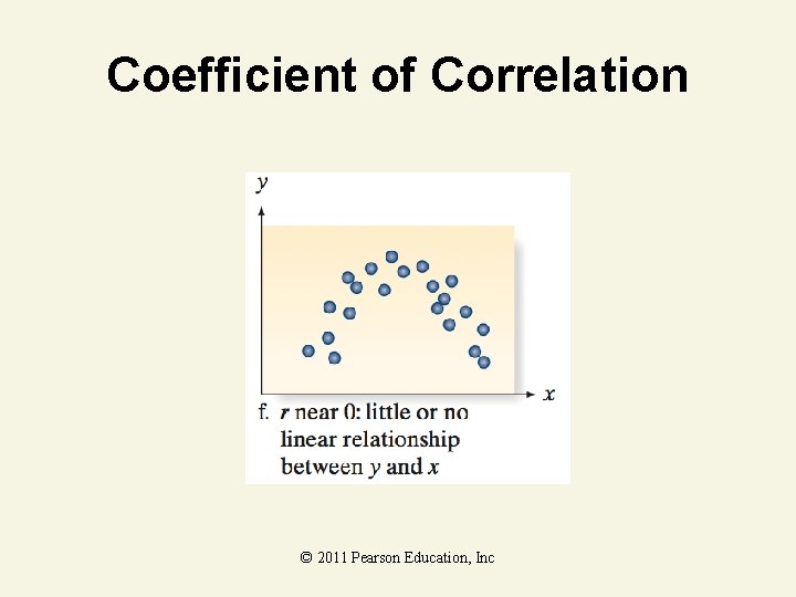
Coefficient of Correlation © 2011 Pearson Education, Inc
Coefficient of Correlation Example You’re a marketing analyst for Hasbro Toys. Ad Expenditure (100$) Sales (Units) 1 1 2 1 3 2 4 2 5 4 Calculate the coefficient of correlation. © 2011 Pearson Education, Inc
Coefficient of Correlation Solution © 2011 Pearson Education, Inc
A Test for Linear Correlation One-Tailed Test H 0: = 0 Ha: < 0 (or Ha: > 0) Rejection region: t > t (or t < –t ) Where the distribution of t depends on (n – 2) degrees of freedom © 2011 Pearson Education, Inc
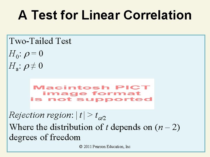
A Test for Linear Correlation Two-Tailed Test H 0: = 0 Ha : ≠ 0 Rejection region: | t | > t Where the distribution of t depends on (n – 2) degrees of freedom © 2011 Pearson Education, Inc
Condition Required for a Valid Test of Correlation The sample of (x, y) values is randomly selected from a normal population. © 2011 Pearson Education, Inc
Coefficient of Correlation Thinking Challenge You’re an economist for the county cooperative. You gather the following data: Fertilizer (lb. ) Yield (lb. ) 4 3. 0 6 5. 5 10 6. 5 12 9. 0 Find the coefficient of correlation. © 1984 -1994 T/Maker Co. © 2011 Pearson Education, Inc
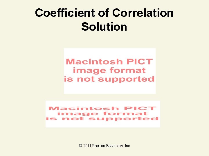
Coefficient of Correlation Solution © 2011 Pearson Education, Inc
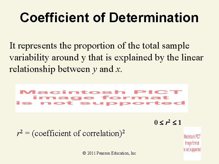
Coefficient of Determination It represents the proportion of the total sample variability around y that is explained by the linear relationship between y and x. 0 r 2 1 r 2 = (coefficient of correlation)2 © 2011 Pearson Education, Inc
Coefficient of Determination Example You’re a marketing analyst for Hasbro Toys. You know r =. 904. Ad Expenditure (100$) Sales (Units) 1 1 2 1 3 2 4 2 5 4 Calculate and interpret the coefficient of determination. © 2011 Pearson Education, Inc
Coefficient of Determination Solution r 2 = (coefficient of correlation)2 r 2 = (. 904)2 r 2 =. 817 Interpretation: About 81. 7% of the sample variation in Sales (y) can be explained by using Ad $ (x) to predict Sales (y) in the linear model. © 2011 Pearson Education, Inc
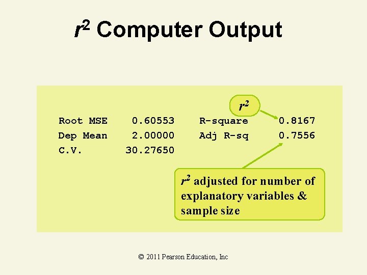
2 r Computer Output r 2 Root MSE Dep Mean C. V. 0. 60553 2. 00000 30. 27650 R-square Adj R-sq 0. 8167 0. 7556 r 2 adjusted for number of explanatory variables & sample size © 2011 Pearson Education, Inc
10. 6 Using the Model for Estimation and Determination © 2011 Pearson Education, Inc
Regression Modeling Steps 1. Hypothesize deterministic component 2. Estimate unknown model parameters 3. Specify probability distribution of random error term • Estimate standard deviation of error 4. Evaluate model 5. Use model for prediction and estimation © 2011 Pearson Education, Inc
Prediction With Regression Models • Types of predictions – Point estimates – Interval estimates • What is predicted – Population mean response E(y) for given x § Point on population regression line – Individual response (yi) for given x © 2011 Pearson Education, Inc
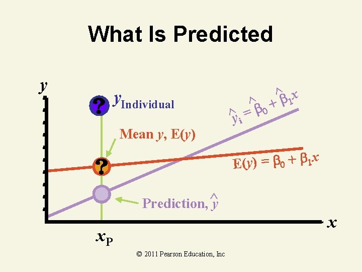
What Is Predicted y y. Individual ^y i ^ = b 0 x ^ b 1 + Mean y, E(y) = b 0 + b 1 x Prediction, ^ y x x. P © 2011 Pearson Education, Inc
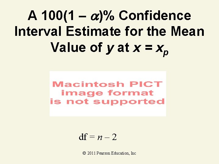
A 100(1 – )% Confidence Interval Estimate for the Mean Value of y at x = xp df = n – 2 © 2011 Pearson Education, Inc
Factors Affecting Interval Width 1. Level of confidence (1 – ) • Width increases as confidence increases 2. Data dispersion (s) • Width increases as variation increases 3. Sample size • Width decreases as sample size increases 4. Distance of xp from mean x 1. Width increases as distance increases © 2011 Pearson Education, Inc
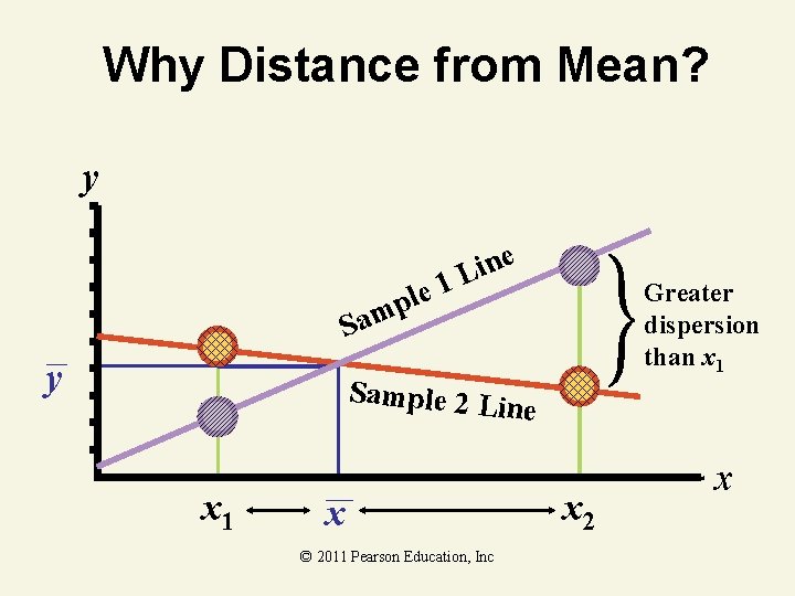
Why Distance from Mean? y 1 e l p e n i L Greater dispersion than x 1 Sam y Sample 2 L in x 1 x © 2011 Pearson Education, Inc e x 2 x
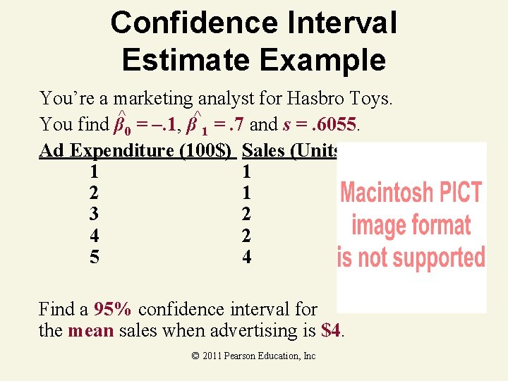
Confidence Interval Estimate Example You’re a marketing analyst for Hasbro Toys. You find β^0 = –. 1, β^1 =. 7 and s =. 6055. Ad Expenditure (100$) Sales (Units) 1 1 2 1 3 2 4 2 5 4 Find a 95% confidence interval for the mean sales when advertising is $4. © 2011 Pearson Education, Inc
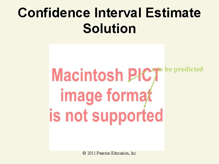
Confidence Interval Estimate Solution x to be predicted © 2011 Pearson Education, Inc
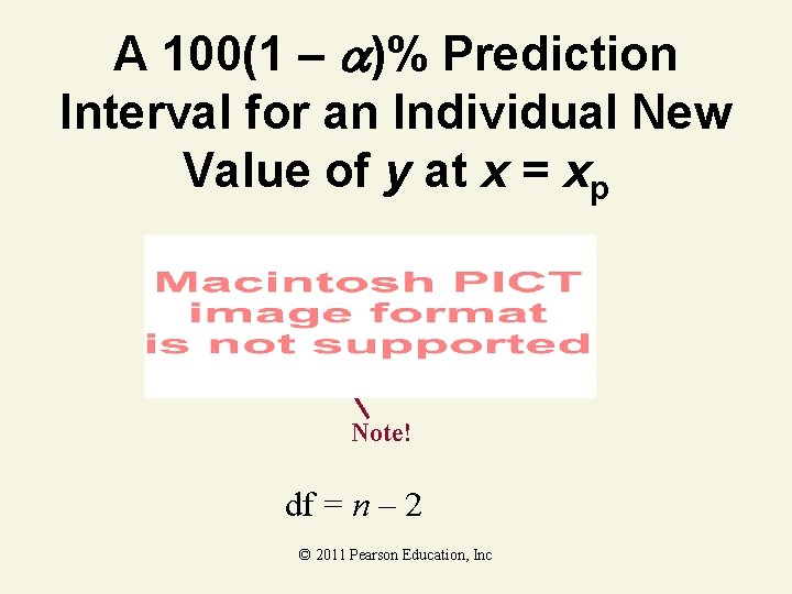
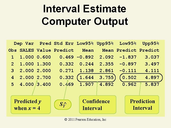
A 100(1 – )% Prediction Interval for an Individual New Value of y at x = xp Note! df = n – 2 © 2011 Pearson Education, Inc
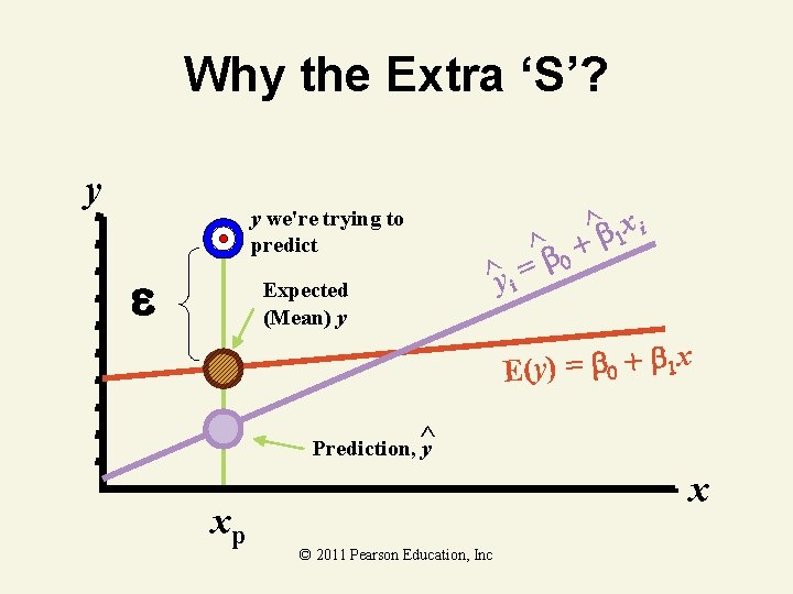
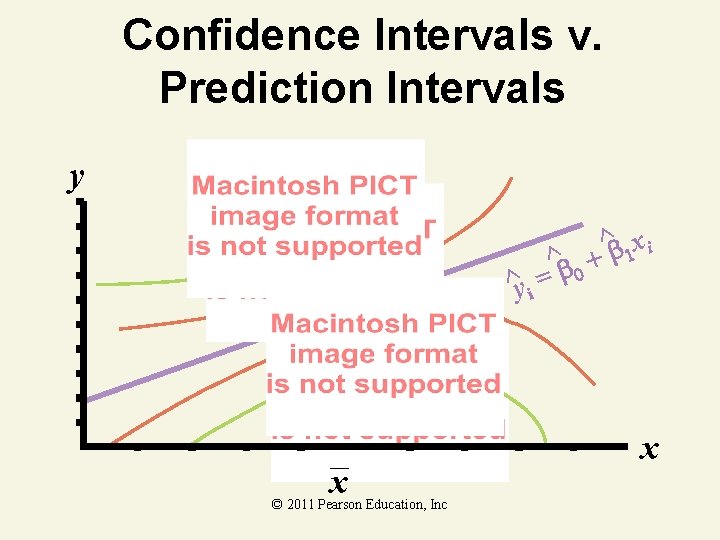
Why the Extra ‘S’? y y we're trying to predict e Expected (Mean) y ^y i ^ = b 0 xi ^ b 1 + E(y) = b 0 + b 1 x Prediction, ^ y xp x © 2011 Pearson Education, Inc
Prediction Interval Example You’re a marketing analyst for Hasbro Toys. You find β^0 = –. 1, β^ 1 =. 7 and s =. 6055. Ad Expenditure (1000$) Sales (Units) 1 1 2 1 3 2 4 2 5 4 Predict the sales when advertising is $400. Use a 95% prediction interval. © 2011 Pearson Education, Inc
Prediction Interval Solution x to be predicted © 2011 Pearson Education, Inc
Interval Estimate Computer Output Dep Var Obs SALES 1 1. 000 2 1. 000 3 2. 000 4 2. 000 5 4. 000 Pred Std Err Low 95% Upp 95% Value Predict Mean Predict 0. 600 0. 469 -0. 892 2. 092 -1. 837 3. 037 1. 300 0. 332 0. 244 2. 355 -0. 897 3. 497 2. 000 0. 271 1. 138 2. 861 -0. 111 4. 111 2. 700 0. 332 1. 644 3. 755 0. 502 4. 897 3. 400 0. 469 1. 907 4. 892 0. 962 5. 837 Predicted y when x = 4 SY^ Confidence Interval © 2011 Pearson Education, Inc Prediction Interval
Confidence Intervals v. Prediction Intervals y ^y i x © 2011 Pearson Education, Inc ^ = b 0 xi ^ b 1 + x
10. 7 A Complete Example © 2011 Pearson Education, Inc
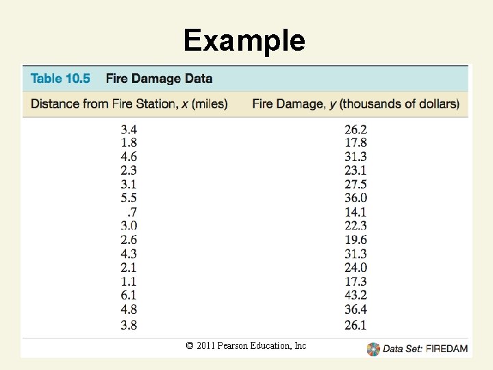
Example Suppose a fire insurance company wants to relate the amount of fire damage in major residential fires to the distance between the burning house and the nearest fire station. The study is to be conducted in a large suburb of a major city; a sample of 15 recent fires in this suburb is selected. The amount of damage, y, and the distance between the fire and the nearest fire station, x, are recorded for each fire. © 2011 Pearson Education, Inc
Example © 2011 Pearson Education, Inc
Example Step 1: First, we hypothesize a model to relate fire damage, y, to the distance from the nearest fire station, x. We hypothesize a straight-line probabilistic model: y = 0 + 1 x + © 2011 Pearson Education, Inc
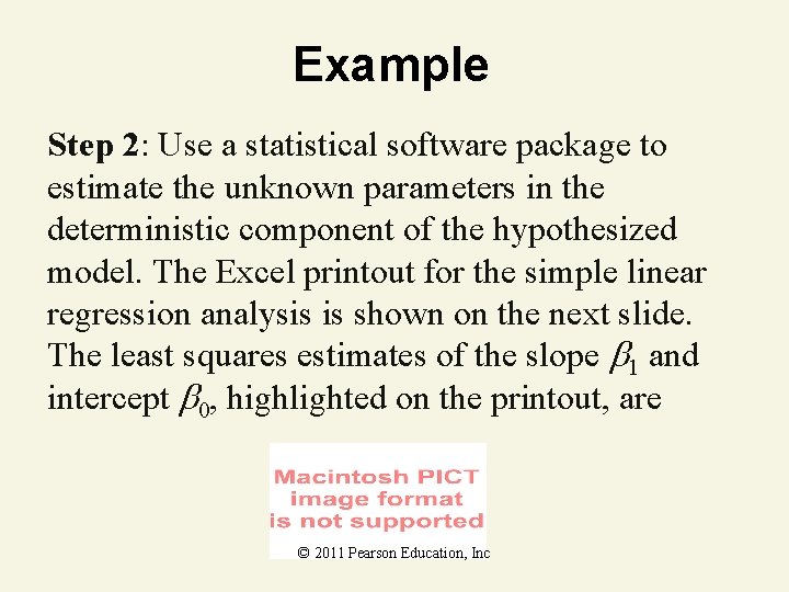
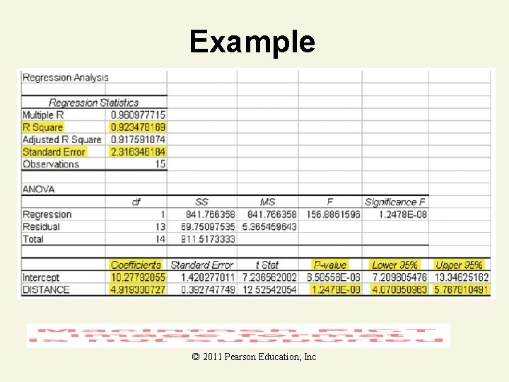
Example Step 2: Use a statistical software package to estimate the unknown parameters in the deterministic component of the hypothesized model. The Excel printout for the simple linear regression analysis is shown on the next slide. The least squares estimates of the slope 1 and intercept 0, highlighted on the printout, are © 2011 Pearson Education, Inc
Example © 2011 Pearson Education, Inc
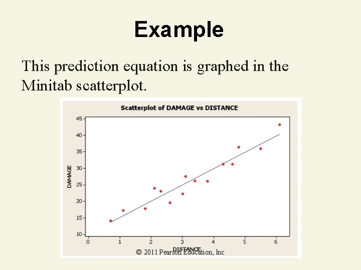
Example This prediction equation is graphed in the Minitab scatterplot. © 2011 Pearson Education, Inc
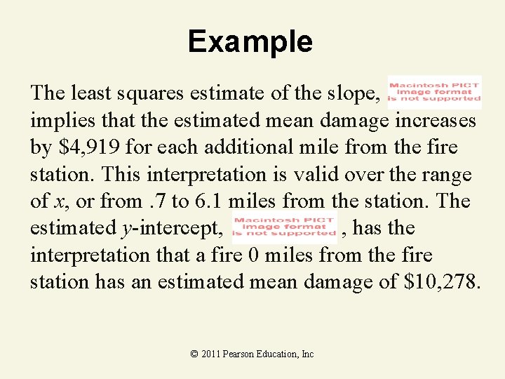
Example The least squares estimate of the slope, implies that the estimated mean damage increases by $4, 919 for each additional mile from the fire station. This interpretation is valid over the range of x, or from. 7 to 6. 1 miles from the station. The estimated y-intercept, , has the interpretation that a fire 0 miles from the fire station has an estimated mean damage of $10, 278. © 2011 Pearson Education, Inc
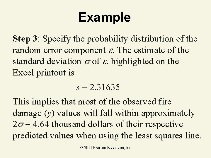
Example Step 3: Specify the probability distribution of the random error component . The estimate of the standard deviation of , highlighted on the Excel printout is s = 2. 31635 This implies that most of the observed fire damage (y) values will fall within approximately 2 = 4. 64 thousand dollars of their respective predicted values when using the least squares line. © 2011 Pearson Education, Inc
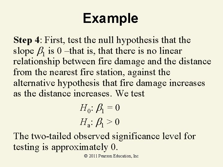
Example Step 4: First, test the null hypothesis that the slope 1 is 0 –that is, that there is no linear relationship between fire damage and the distance from the nearest fire station, against the alternative hypothesis that fire damage increases as the distance increases. We test H 0: 1 = 0 Ha : 1 > 0 The two-tailed observed significance level for testing is approximately 0. © 2011 Pearson Education, Inc
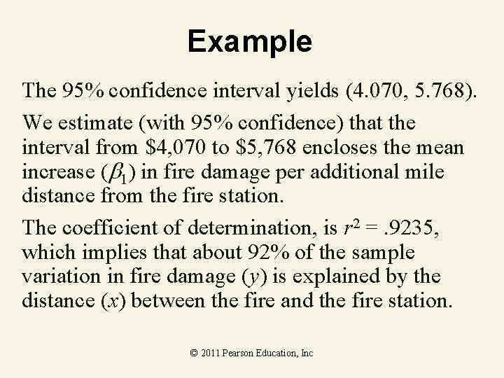
Example The 95% confidence interval yields (4. 070, 5. 768). We estimate (with 95% confidence) that the interval from $4, 070 to $5, 768 encloses the mean increase ( 1) in fire damage per additional mile distance from the fire station. The coefficient of determination, is r 2 =. 9235, which implies that about 92% of the sample variation in fire damage (y) is explained by the distance (x) between the fire and the fire station. © 2011 Pearson Education, Inc
Example The coefficient of correlation, r, that measures the strength of the linear relationship between y and x is not shown on the Excel printout and must be calculated. We find The high correlation confirms our conclusion that 1 is greater than 0; it appears that fire damage and distance from the fire station are positively correlated. All signs point to a strong linear relationship between y and x. © 2011 Pearson Education, Inc
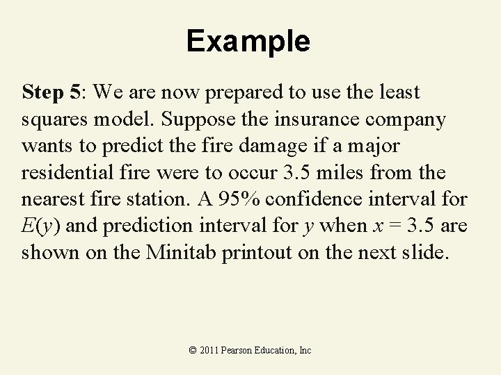
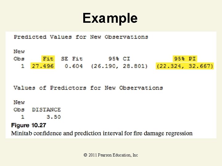
Example Step 5: We are now prepared to use the least squares model. Suppose the insurance company wants to predict the fire damage if a major residential fire were to occur 3. 5 miles from the nearest fire station. A 95% confidence interval for E(y) and prediction interval for y when x = 3. 5 are shown on the Minitab printout on the next slide. © 2011 Pearson Education, Inc
Example Step 5: We are now prepared to use the least © 2011 Pearson Education, Inc
Example The predicted value (highlighted on the printout) is , while the 95% prediction interval (also highlighted) is (22. 3239, 32. 6672). Therefore, with 95% confidence we predict fire damage in a major residential fire 3. 5 miles from the nearest station to be between $22, 324 and $32, 667. © 2011 Pearson Education, Inc
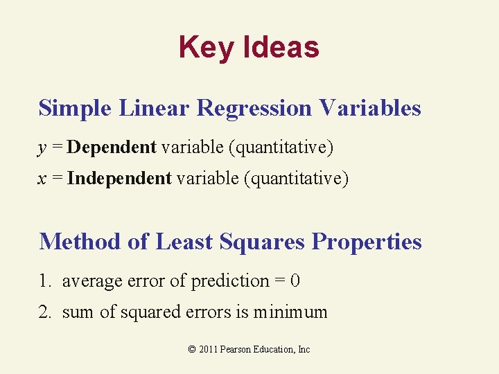
Key Ideas Simple Linear Regression Variables y = Dependent variable (quantitative) x = Independent variable (quantitative) Method of Least Squares Properties 1. average error of prediction = 0 2. sum of squared errors is minimum © 2011 Pearson Education, Inc
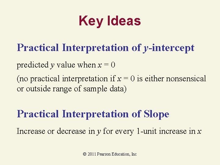
Key Ideas Practical Interpretation of y-intercept predicted y value when x = 0 (no practical interpretation if x = 0 is either nonsensical or outside range of sample data) Practical Interpretation of Slope Increase or decrease in y for every 1 -unit increase in x © 2011 Pearson Education, Inc
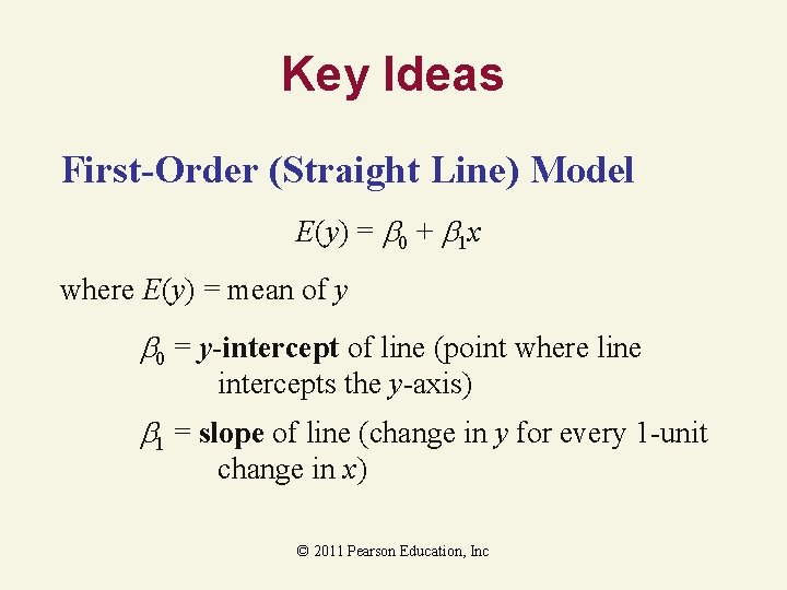
Key Ideas First-Order (Straight Line) Model E(y) = 0 + 1 x where E(y) = mean of y 0 = y-intercept of line (point where line intercepts the y-axis) 1 = slope of line (change in y for every 1 -unit change in x) © 2011 Pearson Education, Inc
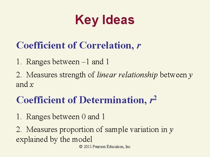
Key Ideas Coefficient of Correlation, r 1. Ranges between – 1 and 1 2. Measures strength of linear relationship between y and x Coefficient of Determination, r 2 1. Ranges between 0 and 1 2. Measures proportion of sample variation in y explained by the model © 2011 Pearson Education, Inc
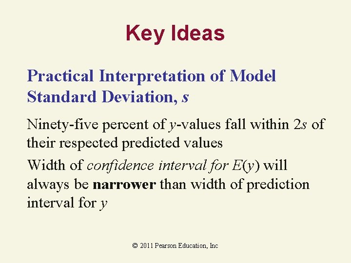
Key Ideas Practical Interpretation of Model Standard Deviation, s Ninety-five percent of y-values fall within 2 s of their respected predicted values Width of confidence interval for E(y) will always be narrower than width of prediction interval for y © 2011 Pearson Education, Inc
- Slides: 106