2011 Pearson Education Inc Statistics for Business and
© 2011 Pearson Education, Inc
Statistics for Business and Economics Chapter 4 Random Variables & Probability Distributions © 2011 Pearson Education, Inc
Content 1. Two Types of Random Variables 2. Probability Distributions for Discrete Random Variables 3. The Binomial Distribution 4. Poisson and Hypergeometric Distributions 5. Probability Distributions for Continuous Random Variables 6. The Normal Distribution © 2011 Pearson Education, Inc
Content (continued) 7. Descriptive Methods for Assessing Normality 8. Approximating a Binomial Distribution with a Normal Distribution 9. Uniform and Exponential Distributions 10. Sampling Distributions 11. The Sampling Distribution of a Sample Mean and the Central Limit Theorem © 2011 Pearson Education, Inc
Learning Objectives 1. Develop the notion of a random variable 2. Learn that numerical data are observed values of either discrete or continuous random variables 3. Study two important types of random variables and their probability models: the binomial and normal model 4. Define a sampling distribution as the probability of a sample statistic 5. Learn that the sampling distribution of follows a normal model © 2011 Pearson Education, Inc

Thinking Challenge • You’re taking a 33 question multiple choice test. Each question has 4 choices. Clueless on 1 question, you decide to guess. What’s the chance you’ll get it right? • If you guessed on all 33 questions, what would be your grade? Would you pass? © 2011 Pearson Education, Inc
4. 1 Two Types of Random Variables © 2011 Pearson Education, Inc
Random Variable A random variable is a variable that assumes numerical values associated with the random outcomes of an experiment, where one (and only one) numerical value is assigned to each sample point. © 2011 Pearson Education, Inc
Discrete Random Variable Random variables that can assume a countable number (finite or infinite) of values are called discrete. © 2011 Pearson Education, Inc
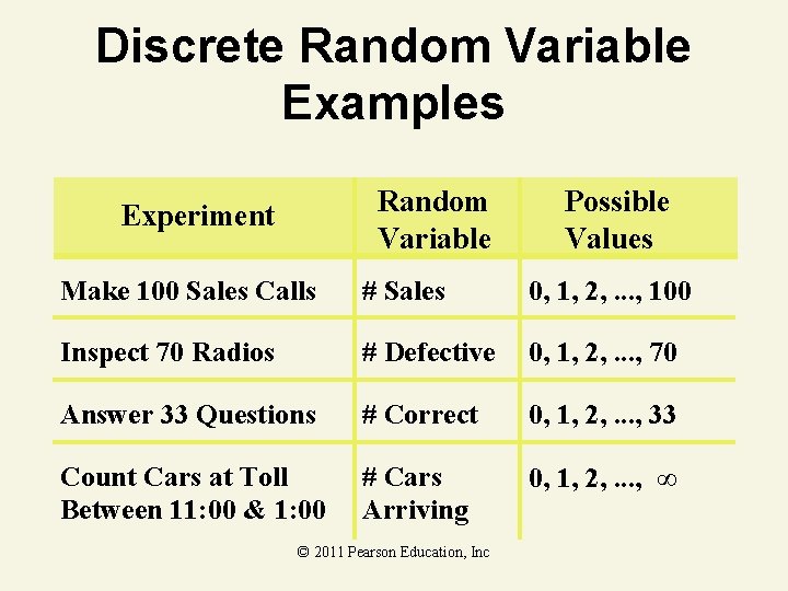
Discrete Random Variable Examples Random Variable Experiment Possible Values Make 100 Sales Calls # Sales 0, 1, 2, . . . , 100 Inspect 70 Radios # Defective 0, 1, 2, . . . , 70 Answer 33 Questions # Correct 0, 1, 2, . . . , 33 Count Cars at Toll Between 11: 00 & 1: 00 # Cars Arriving 0, 1, 2, . . . , ∞ © 2011 Pearson Education, Inc
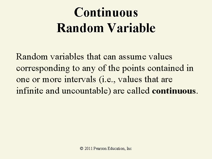
Continuous Random Variable Random variables that can assume values corresponding to any of the points contained in one or more intervals (i. e. , values that are infinite and uncountable) are called continuous. © 2011 Pearson Education, Inc
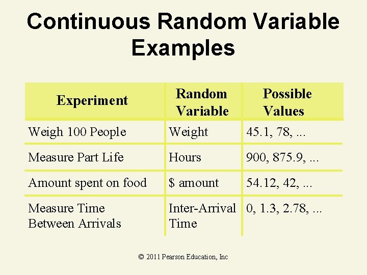
Continuous Random Variable Examples Random Variable Experiment Possible Values Weigh 100 People Weight 45. 1, 78, . . . Measure Part Life Hours 900, 875. 9, . . . Amount spent on food $ amount 54. 12, 42, . . . Measure Time Between Arrivals Inter-Arrival 0, 1. 3, 2. 78, . . . Time © 2011 Pearson Education, Inc
4. 2 Probability Distributions for Discrete Random Variables © 2011 Pearson Education, Inc
Discrete Probability Distribution The probability distribution of a discrete random variable is a graph, table, or formula that specifies the probability associated with each possible value the random variable can assume. © 2011 Pearson Education, Inc
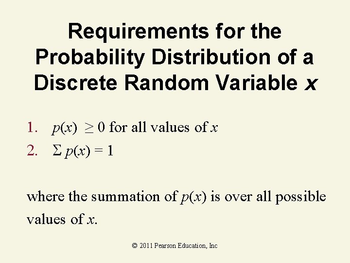
Requirements for the Probability Distribution of a Discrete Random Variable x 1. p(x) ≥ 0 for all values of x . p(x) = 1 where the summation of p(x) is over all possible values of x. © 2011 Pearson Education, Inc
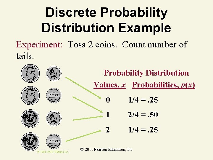
Discrete Probability Distribution Example Experiment: Toss 2 coins. Count number of tails. Probability Distribution Values, x Probabilities, p(x) © 1984 -1994 T/Maker Co. 0 1/4 =. 25 1 2/4 =. 50 2 1/4 =. 25 © 2011 Pearson Education, Inc
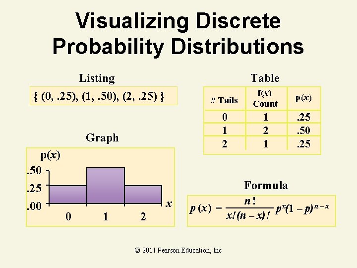
Visualizing Discrete Probability Distributions Listing Table { (0, . 25), (1, . 50), (2, . 25) } # Tails f(x) Count p(x) 0 1 2 1 . 25. 50. 25 Graph p(x). 50. 25. 00 Formula x 0 1 2 p (x ) = © 2011 Pearson Education, Inc n! px(1 – p)n – x x!(n – x)!
Summary Measures 1. Expected Value (Mean of probability distribution) • Weighted average of all possible values • = E(x) = x p(x) • Variance • Weighted average of squared deviation about mean • 2 = E[(x p(x) 3. Standard Deviation ● © 2011 Pearson Education, Inc
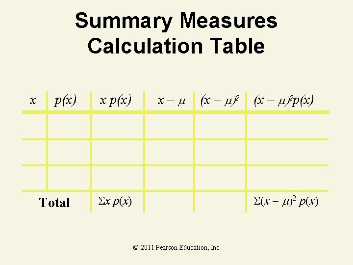
Summary Measures Calculation Table x p(x) Total x p(x) x– (x – )2 p(x) (x p(x) x p(x) © 2011 Pearson Education, Inc

Thinking Challenge You toss 2 coins. You’re interested in the number of tails. What are the expected value, variance, and standard deviation of this random variable, number of tails? © 1984 -1994 T/Maker Co. © 2011 Pearson Education, Inc
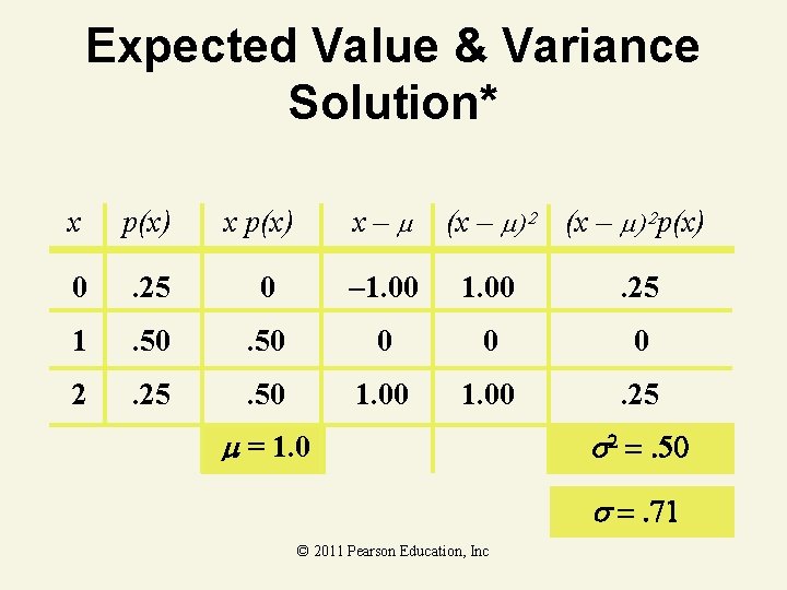
Expected Value & Variance Solution* x p(x) x– (x – ) 2 p(x) 0 . 25 0 – 1. 00 . 25 1 . 50 0 0 0 2 . 25 . 50 1. 00 . 25 = 1. 0 2 =. 50 =. 71 © 2011 Pearson Education, Inc
Probability Rules for Discrete Random Variables Let x be a discrete random variable with probability distribution p(x), mean µ, and standard deviation . Then, depending on the shape of p(x), the following probability statements can be made: Chebyshev’s Rule © 2011 Pearson Education, Inc Empirical Rule
4. 3 The Binomial Distribution © 2011 Pearson Education, Inc
Binomial Distribution Number of ‘successes’ in a sample of n observations (trials) • Number of reds in 15 spins of roulette wheel • Number of defective items in a batch of 5 items • Number correct on a 33 question exam • Number of customers who purchase out of 100 customers who enter store (each customer is equally likely to pyrchase) © 2011 Pearson Education, Inc
Binomial Probability Characteristics of a Binomial Experiment 1. The experiment consists of n identical trials. 2. There are only two possible outcomes on each trial. We will denote one outcome by S (for success) and the other by F (for failure). 3. The probability of S remains the same from trial to trial. This probability is denoted by p, and the probability of F is denoted by q. Note that q = 1 – p. 4. The trials are independent. 5. The binomial random variable x is the number of S’s in n trials. © 2011 Pearson Education, Inc
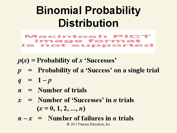
Binomial Probability Distribution p(x) = Probability of x ‘Successes’ p = Probability of a ‘Success’ on a single trial q = 1–p n = Number of trials x = Number of ‘Successes’ in n trials (x = 0, 1, 2, . . . , n) n – x = Number of failures in n trials © 2011 Pearson Education, Inc
Binomial Probability Distribution Example Experiment: Toss 1 coin 5 times in a row. Note number of tails. What’s the probability of 3 tails? © 1984 -1994 T/Maker Co. © 2011 Pearson Education, Inc
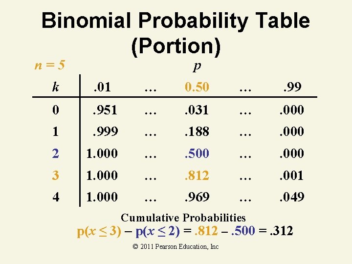
Binomial Probability Table (Portion) n=5 p k . 01 … 0. 50 … . 99 0 . 951 … . 031 … . 000 1 . 999 … . 188 … . 000 2 1. 000 … . 500 … . 000 3 1. 000 … . 812 … . 001 4 1. 000 … . 969 … . 049 Cumulative Probabilities p(x ≤ 3) – p(x ≤ 2) =. 812 –. 500 =. 312 © 2011 Pearson Education, Inc
Binomial Distribution Characteristics n = 5 p = 0. 1 Mean Standard Deviation n = 5 p = 0. 5 © 2011 Pearson Education, Inc
Binomial Distribution Thinking Challenge You’re a telemarketer selling service contracts for Macy’s. You’ve sold 20 in your last 100 calls (p =. 20). If you call 12 people tonight, what’s the probability of A. No sales? B. Exactly 2 sales? C. At most 2 sales? D. At least 2 sales? © 2011 Pearson Education, Inc
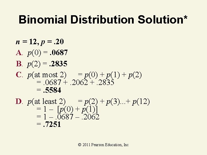
Binomial Distribution Solution* n = 12, p =. 20 A. p(0) =. 0687 B. p(2) =. 2835 C. p(at most 2) = p(0) + p(1) + p(2) =. 0687 +. 2062 +. 2835 =. 5584 D. p(at least 2) = p(2) + p(3). . . + p(12) = 1 – [p(0) + p(1)] = 1 –. 0687 –. 2062 =. 7251 © 2011 Pearson Education, Inc
4. 4 Other Discrete Distributions: Poisson and Hypergeometric © 2011 Pearson Education, Inc
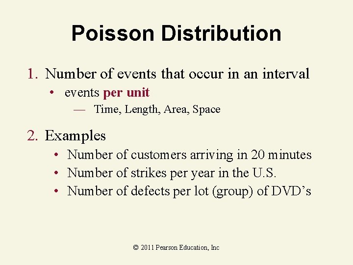
Poisson Distribution 1. Number of events that occur in an interval • events per unit — Time, Length, Area, Space 2. Examples • Number of customers arriving in 20 minutes • Number of strikes per year in the U. S. • Number of defects per lot (group) of DVD’s © 2011 Pearson Education, Inc
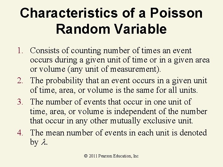
Characteristics of a Poisson Random Variable 1. Consists of counting number of times an event occurs during a given unit of time or in a given area or volume (any unit of measurement). 2. The probability that an event occurs in a given unit of time, area, or volume is the same for all units. 3. The number of events that occur in one unit of time, area, or volume is independent of the number that occur in any other mutually exclusive unit. 4. The mean number of events in each unit is denoted by © 2011 Pearson Education, Inc
Poisson Probability Distribution Function x – p (x ) e x! (x = 0, 1, 2, 3, . . . ) p(x) = = e = x = Probability of x given Mean (expected) number of events in unit 2. 71828. . . (base of natural logarithm) Number of events per unit © 2011 Pearson Education, Inc
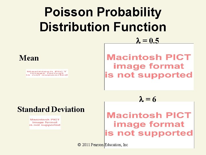
Poisson Probability Distribution Function = 0. 5 Mean = 6 Standard Deviation © 2011 Pearson Education, Inc
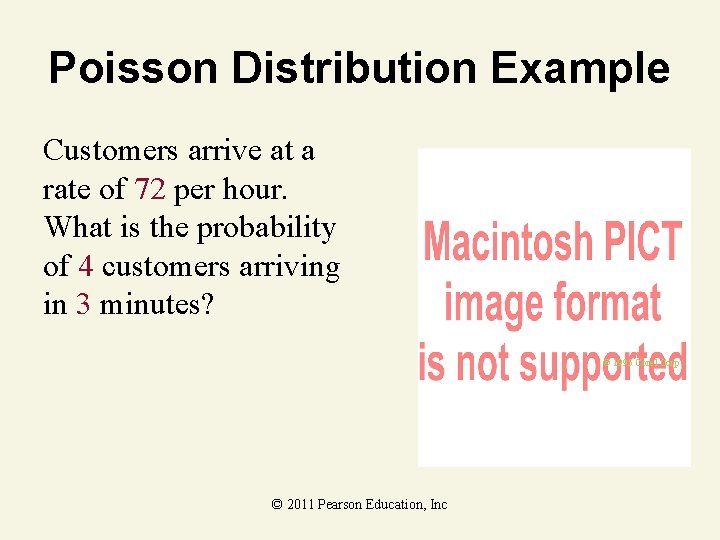
Poisson Distribution Example Customers arrive at a rate of 72 per hour. What is the probability of 4 customers arriving in 3 minutes? © 1995 Corel Corp. © 2011 Pearson Education, Inc
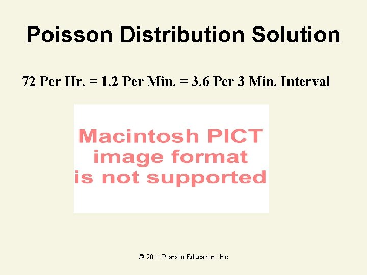
Poisson Distribution Solution 72 Per Hr. = 1. 2 Per Min. = 3. 6 Per 3 Min. Interval © 2011 Pearson Education, Inc
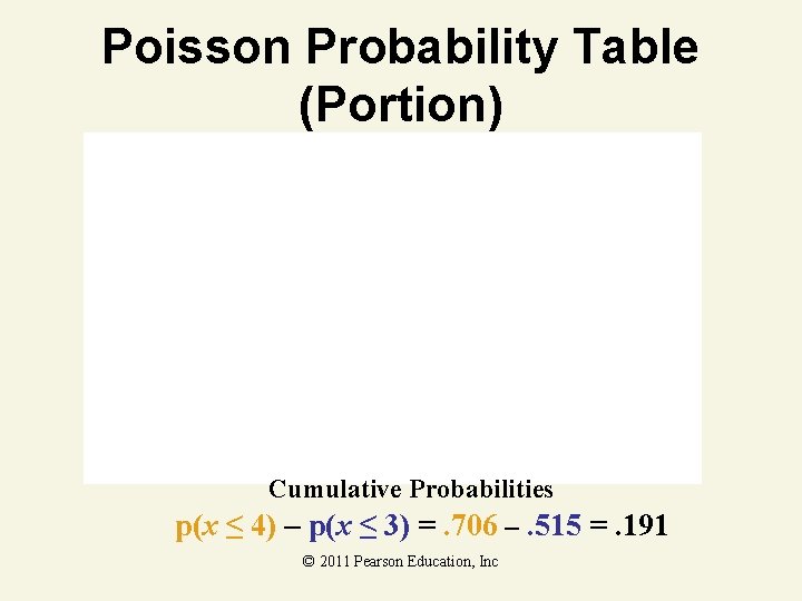
Poisson Probability Table (Portion) Cumulative Probabilities p(x ≤ 4) – p(x ≤ 3) =. 706 –. 515 =. 191 © 2011 Pearson Education, Inc
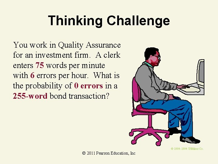
Thinking Challenge You work in Quality Assurance for an investment firm. A clerk enters 75 words per minute with 6 errors per hour. What is the probability of 0 errors in a 255 -word bond transaction? © 1984 -1994 T/Maker Co. © 2011 Pearson Education, Inc
Poisson Distribution Solution: Finding * • 75 words/min = (75 words/min)(60 min/hr) = 4500 words/hr • 6 errors/hr = 6 errors/4500 words =. 00133 errors/word • In a 255 -word transaction (interval): = (. 00133 errors/word )(255 words) =. 34 errors/255 -word transaction © 2011 Pearson Education, Inc
Poisson Distribution Solution: Finding p(0)* © 2011 Pearson Education, Inc
Characteristics of a Hypergeometric Random Variable 1. The experiment consists of randomly drawing n elements without replacement from a set of N elements, r of which are S’s (for success) and (N – r) of which are F’s (for failure). 2. The hypergeometric random variable x is the number of S’s in the draw of n elements. © 2011 Pearson Education, Inc
Hypergeometric Probability Distribution Function [x = Maximum [0, n – (N – r), …, Minimum (r, n)] where. . . © 2011 Pearson Education, Inc
Hypergeometric Probability Distribution Function N = Total number of elements r = Number of S’s in the N elements n = Number of elements drawn x = Number of S’s drawn in the n elements © 2011 Pearson Education, Inc
4. 5 Probability Distributions for Continuous Random Variables © 2011 Pearson Education, Inc
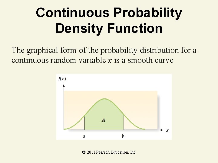
Continuous Probability Density Function The graphical form of the probability distribution for a continuous random variable x is a smooth curve © 2011 Pearson Education, Inc
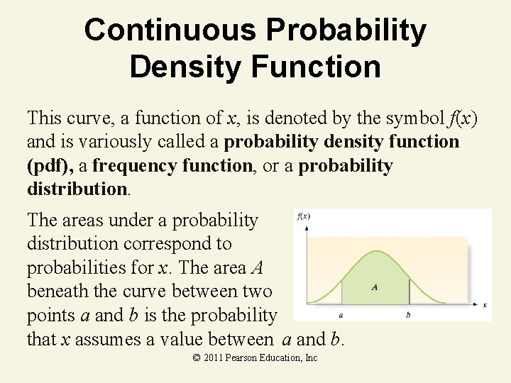
Continuous Probability Density Function This curve, a function of x, is denoted by the symbol f(x) and is variously called a probability density function (pdf), a frequency function, or a probability distribution. The areas under a probability distribution correspond to probabilities for x. The area A beneath the curve between two points a and b is the probability that x assumes a value between a and b. © 2011 Pearson Education, Inc
4. 6 The Normal Distribution © 2011 Pearson Education, Inc
Importance of Normal Distribution 1. Describes many random processes or continuous phenomena 2. Can be used to approximate discrete probability distributions • Example: binomial 3. Basis for classical statistical inference © 2011 Pearson Education, Inc
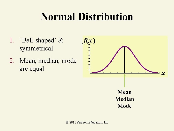
Normal Distribution 1. ‘Bell-shaped’ & symmetrical f(x ) 2. Mean, median, mode are equal x Mean Median Mode © 2011 Pearson Education, Inc
Probability Density Function where µ = Mean of the normal random variable x = Standard deviation π = 3. 1415. . . e = 2. 71828. . . P(x < a) is obtained from a table of normal probabilities © 2011 Pearson Education, Inc
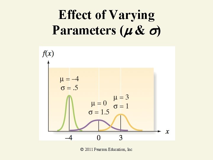
Effect of Varying Parameters ( & ) © 2011 Pearson Education, Inc
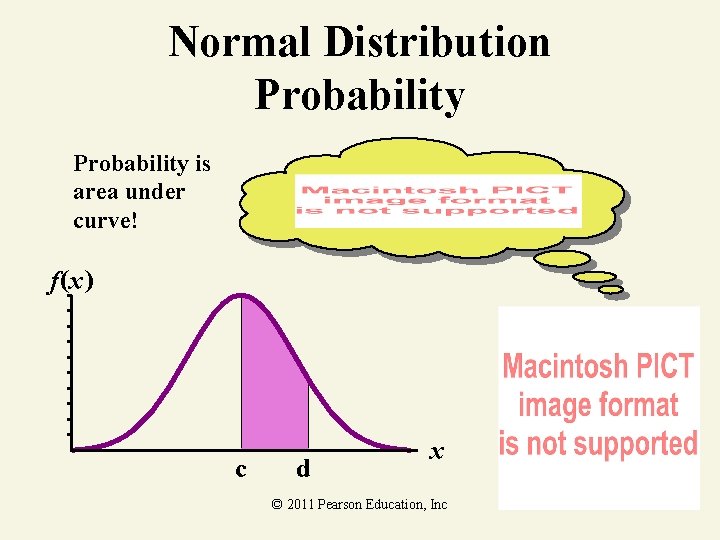
Normal Distribution Probability is area under curve! f(x) c d x © 2011 Pearson Education, Inc
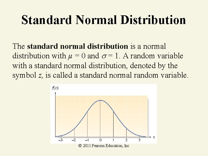
Standard Normal Distribution The standard normal distribution is a normal distribution with µ = 0 and = 1. A random variable with a standard normal distribution, denoted by the symbol z, is called a standard normal random variable. © 2011 Pearson Education, Inc
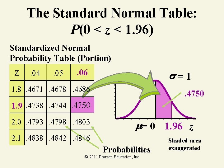
The Standard Normal Table: P(0 < z < 1. 96) Standardized Normal Probability Table (Portion) Z . 04 . 05 . 06 =1 1. 8. 4671. 4678. 4686 . 4750 1. 9. 4738. 4744. 4750 2. 0. 4793. 4798. 4803 = 0 1. 96 z 2. 1. 4838. 4842. 4846 Probabilities © 2011 Pearson Education, Inc Shaded area exaggerated
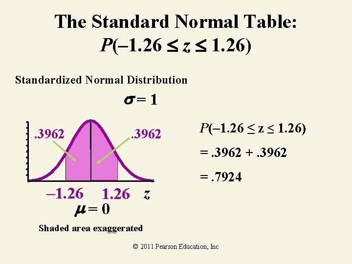
The Standard Normal Table: P(– 1. 26 z 1. 26) Standardized Normal Distribution =1. 3962 P(– 1. 26 ≤ z ≤ 1. 26) =. 3962 +. 3962 1. 26 z =0 – 1. 26 =. 7924 Shaded area exaggerated © 2011 Pearson Education, Inc
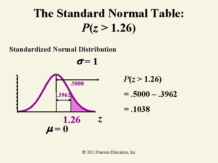
The Standard Normal Table: P(z > 1. 26) Standardized Normal Distribution =1 P(z > 1. 26) . 5000 =. 5000 –. 3962 1. 26 =0 z =. 1038 © 2011 Pearson Education, Inc
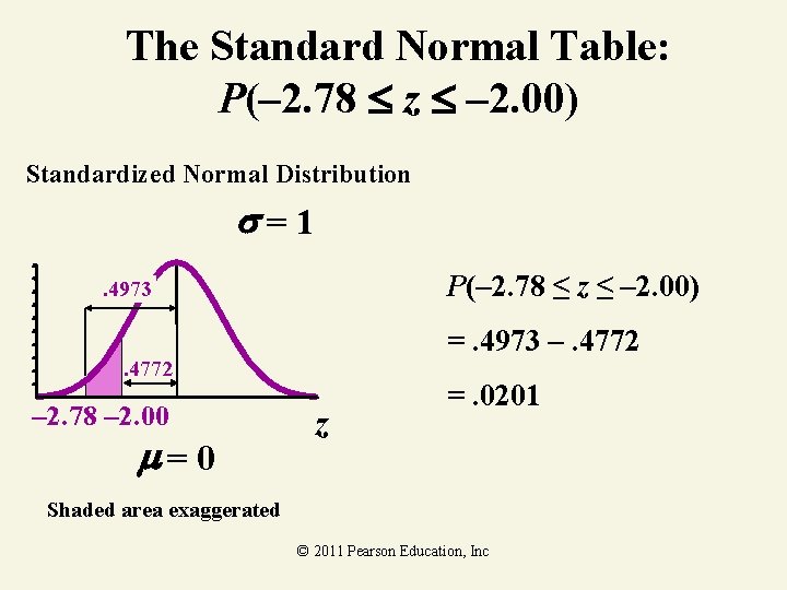
The Standard Normal Table: P(– 2. 78 z – 2. 00) Standardized Normal Distribution =1 P(– 2. 78 ≤ z ≤ – 2. 00) . 4973 =. 4973 –. 4772 – 2. 78 – 2. 00 =0 z =. 0201 Shaded area exaggerated © 2011 Pearson Education, Inc
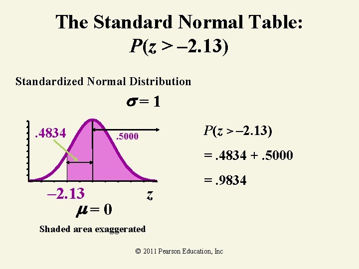
The Standard Normal Table: P(z > – 2. 13) Standardized Normal Distribution =1. 4834 P(z > – 2. 13) . 5000 =. 4834 +. 5000 z – 2. 13 =0 =. 9834 Shaded area exaggerated © 2011 Pearson Education, Inc
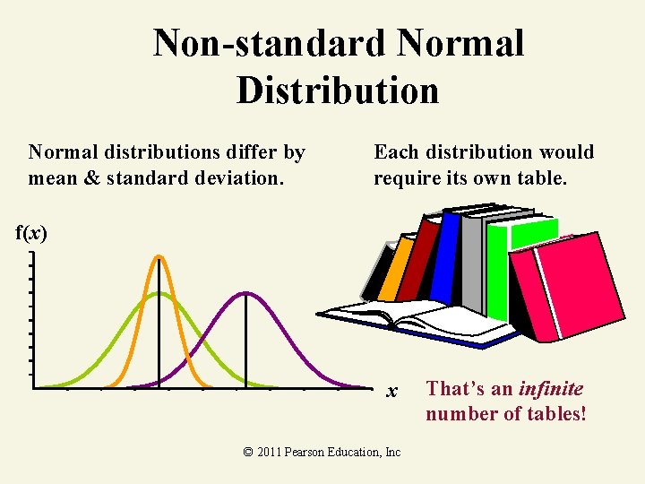
Non-standard Normal Distribution Normal distributions differ by mean & standard deviation. Each distribution would require its own table. f(x) x © 2011 Pearson Education, Inc That’s an infinite number of tables!
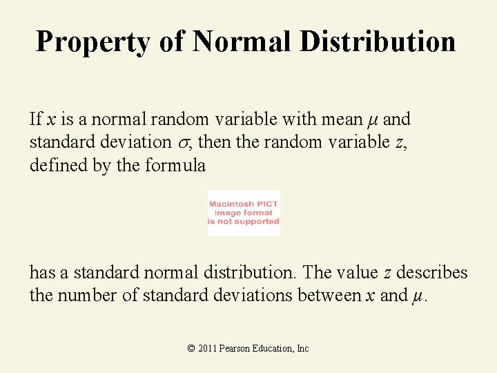
Property of Normal Distribution If x is a normal random variable with mean μ and standard deviation , then the random variable z, defined by the formula has a standard normal distribution. The value z describes the number of standard deviations between x and µ. © 2011 Pearson Education, Inc
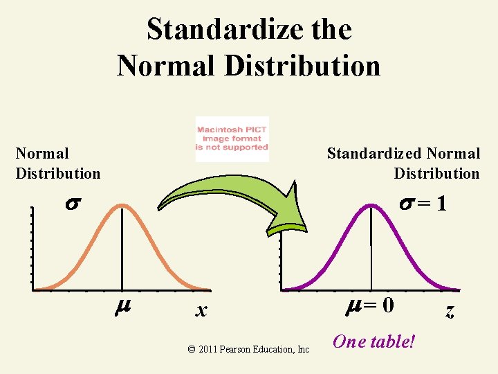
Standardize the Normal Distribution Standardized Normal Distribution = 1 x © 2011 Pearson Education, Inc = 0 One table! z
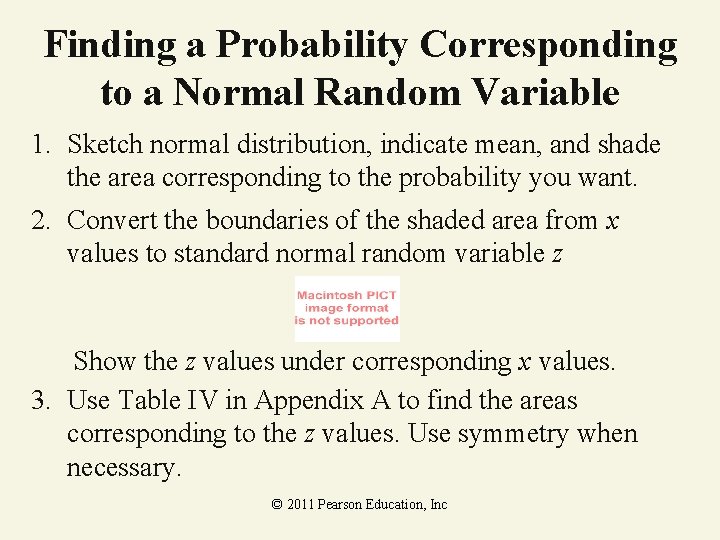
Finding a Probability Corresponding to a Normal Random Variable 1. Sketch normal distribution, indicate mean, and shade the area corresponding to the probability you want. 2. Convert the boundaries of the shaded area from x values to standard normal random variable z Show the z values under corresponding x values. 3. Use Table IV in Appendix A to find the areas corresponding to the z values. Use symmetry when necessary. © 2011 Pearson Education, Inc
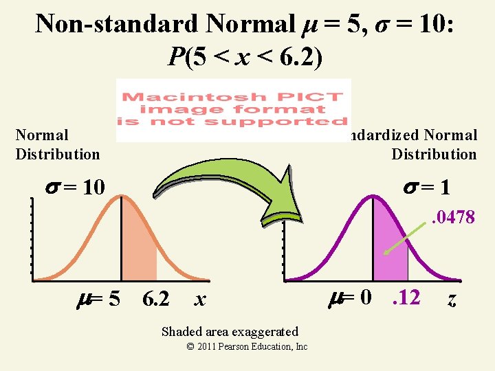
Non-standard Normal μ = 5, σ = 10: P(5 < x < 6. 2) Standardized Normal Distribution = 10 =1. 0478 = 5 6. 2 x Shaded area exaggerated © 2011 Pearson Education, Inc = 0. 12 z
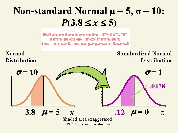
Non-standard Normal μ = 5, σ = 10: P(3. 8 x 5) Normal Distribution Standardized Normal Distribution = 10 =1. 0478 3. 8 = 5 x Shaded area exaggerated © 2011 Pearson Education, Inc -. 12 = 0 z
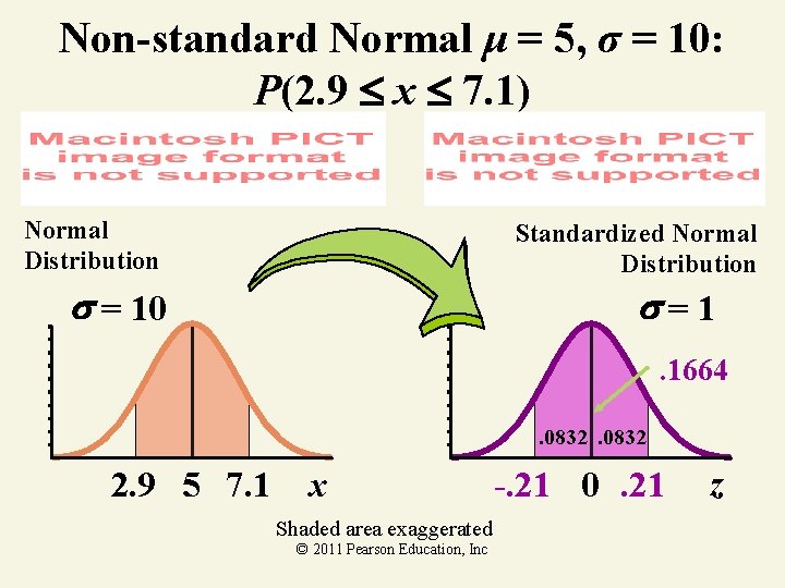
Non-standard Normal μ = 5, σ = 10: P(2. 9 x 7. 1) Normal Distribution Standardized Normal Distribution = 10 =1. 1664. 0832 2. 9 5 7. 1 x Shaded area exaggerated © 2011 Pearson Education, Inc -. 21 0. 21 z
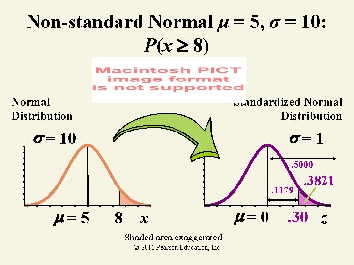
Non-standard Normal μ = 5, σ = 10: P(x 8) Normal Distribution Standardized Normal Distribution = 10 =1. 5000. 1179 =5 8 x Shaded area exaggerated © 2011 Pearson Education, Inc =0 . 3821 . 30 z
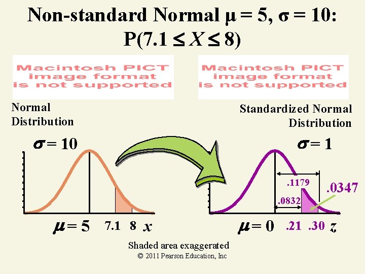
Non-standard Normal μ = 5, σ = 10: P(7. 1 X 8) Normal Distribution Standardized Normal Distribution = 10 =1. 1179. 0832 =5 7. 1 8 x Shaded area exaggerated © 2011 Pearson Education, Inc =0 . 21. 30 . 0347 z
Normal Distribution Thinking Challenge You work in Quality Control for GE. Light bulb life has a normal distribution with = 2000 hours and = 200 hours. What’s the probability that a bulb will last A. between 2000 and 2400 hours? B. less than 1470 hours? © 2011 Pearson Education, Inc
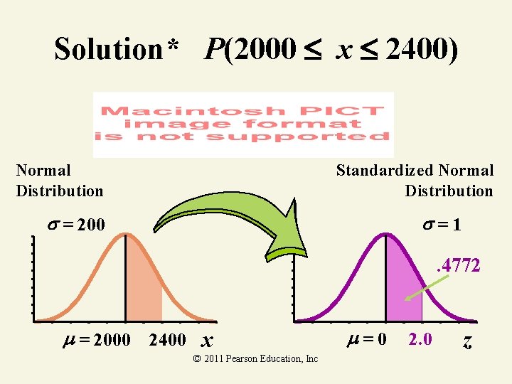
Solution* P(2000 x 2400) Normal Distribution Standardized Normal Distribution = 200 =1 . 4772 = 2000 2400 x © 2011 Pearson Education, Inc =0 2. 0 z
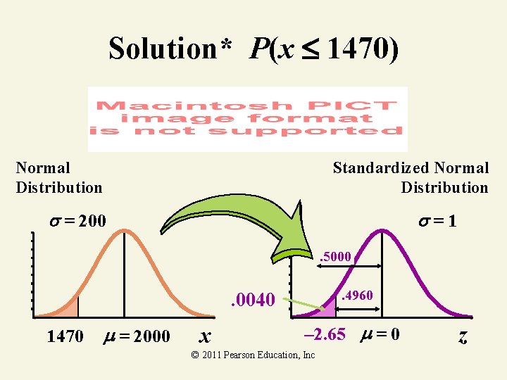
Solution* P(x 1470) Normal Distribution Standardized Normal Distribution = 200 =1. 5000. 4960 . 0040 1470 = 2000 x – 2. 65 = 0 © 2011 Pearson Education, Inc z
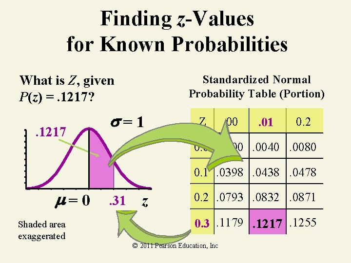
Finding z-Values for Known Probabilities Standardized Normal Probability Table (Portion) What is Z, given P(z) =. 1217? . 1217 =1 Z . 00 . 01 0. 2 0. 0. 0000. 0040. 0080 0. 1. 0398. 0438. 0478 =0 Shaded area exaggerated . 31 ? z 0. 2. 0793. 0832. 0871 0. 3. 1179. 1217. 1255 © 2011 Pearson Education, Inc
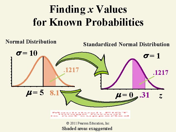
Finding x Values for Known Probabilities Normal Distribution Standardized Normal Distribution = 10 =1. 1217 = 5 8. 1 ? x © 2011 Pearson Education, Inc Shaded areas exaggerated . 1217 = 0. 31 z
4. 7 Descriptive Methods for Assessing Normality © 2011 Pearson Education, Inc
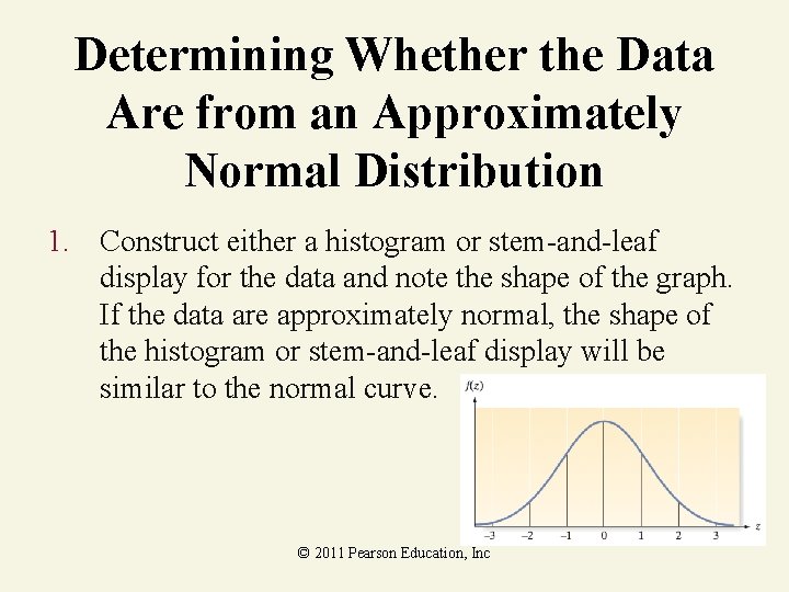
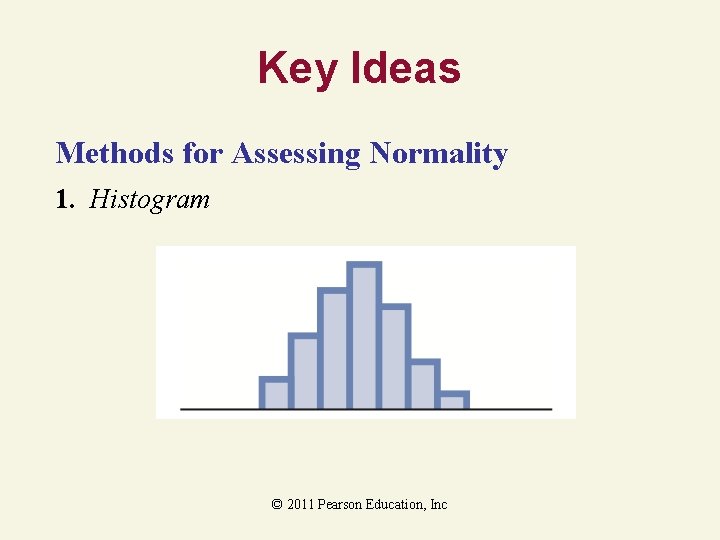
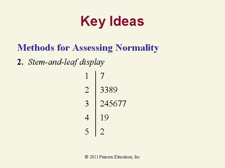
Determining Whether the Data Are from an Approximately Normal Distribution 1. Construct either a histogram or stem-and-leaf display for the data and note the shape of the graph. If the data are approximately normal, the shape of the histogram or stem-and-leaf display will be similar to the normal curve. © 2011 Pearson Education, Inc
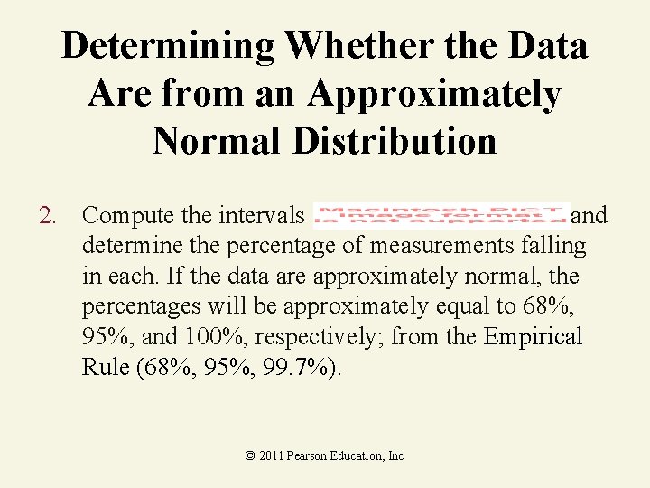
Determining Whether the Data Are from an Approximately Normal Distribution 2. Compute the intervals and determine the percentage of measurements falling in each. If the data are approximately normal, the percentages will be approximately equal to 68%, 95%, and 100%, respectively; from the Empirical Rule (68%, 95%, 99. 7%). © 2011 Pearson Education, Inc
Determining Whether the Data Are from an Approximately Normal Distribution 3. Find the interquartile range, IQR, and standard deviation, s, for the sample, then calculate the ratio IQR/s. If the data are approximately normal, then IQR/s ≈ 1. 3. © 2011 Pearson Education, Inc
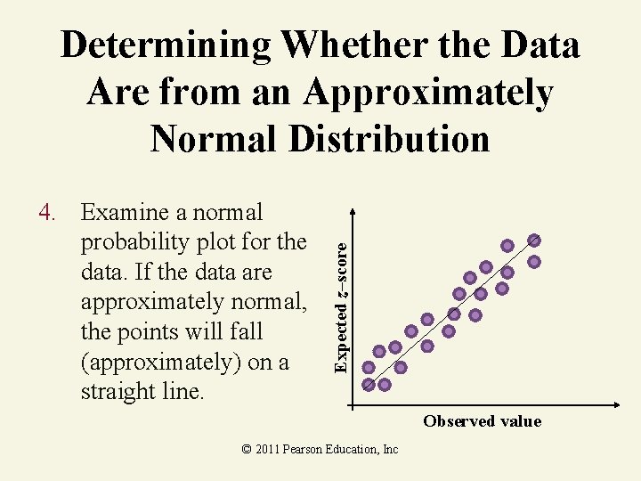
4. Examine a normal probability plot for the data. If the data are approximately normal, the points will fall (approximately) on a straight line. Expected z–score Determining Whether the Data Are from an Approximately Normal Distribution Observed value © 2011 Pearson Education, Inc
Normal Probability Plot A normal probability plot for a data set is a scatterplot with the ranked data values on one axis and their corresponding expected z-scores from a standard normal distribution on the other axis. [Note: Computation of the expected standard normal z-scores are beyond the scope of this text. Therefore, we will rely on available statistical software packages to generate a normal probability plot. ] © 2011 Pearson Education, Inc
4. 8 Approximating a Binomial Distribution with a Normal Distribution © 2011 Pearson Education, Inc
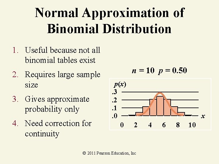
Normal Approximation of Binomial Distribution 1. Useful because not all binomial tables exist 2. Requires large sample size 3. Gives approximate probability only 4. Need correction for continuity n = 10 p = 0. 50 p(x). 3. 2. 1. 0 0 x 2 © 2011 Pearson Education, Inc 4 6 8 10
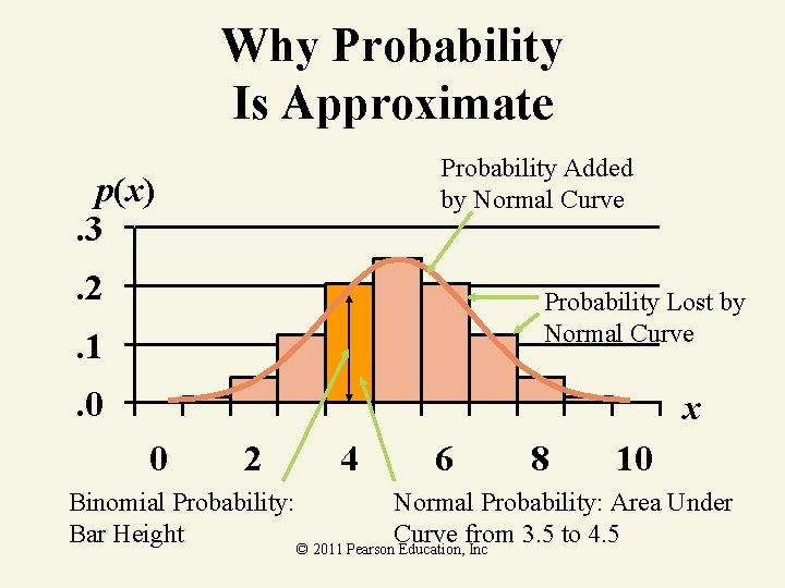
Why Probability Is Approximate Probability Added by Normal Curve p(x). 3. 2 Probability Lost by Normal Curve . 1. 0 x 0 2 4 6 8 10 Binomial Probability: Normal Probability: Area Under Bar Height Curve from 3. 5 to 4. 5 © 2011 Pearson Education, Inc
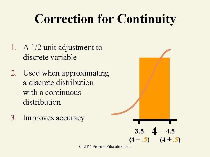
Correction for Continuity 1. A 1/2 unit adjustment to discrete variable 2. Used when approximating a discrete distribution with a continuous distribution 3. Improves accuracy 3. 5 (4 –. 5) © 2011 Pearson Education, Inc 4 4. 5 (4 +. 5)
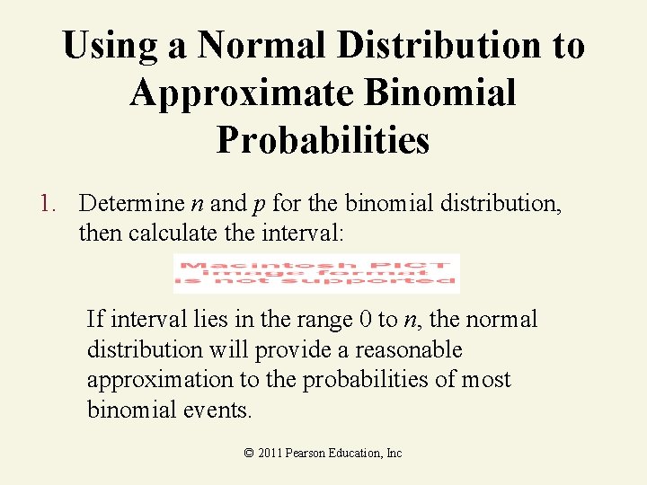
Using a Normal Distribution to Approximate Binomial Probabilities 1. Determine n and p for the binomial distribution, then calculate the interval: If interval lies in the range 0 to n, the normal distribution will provide a reasonable approximation to the probabilities of most binomial events. © 2011 Pearson Education, Inc
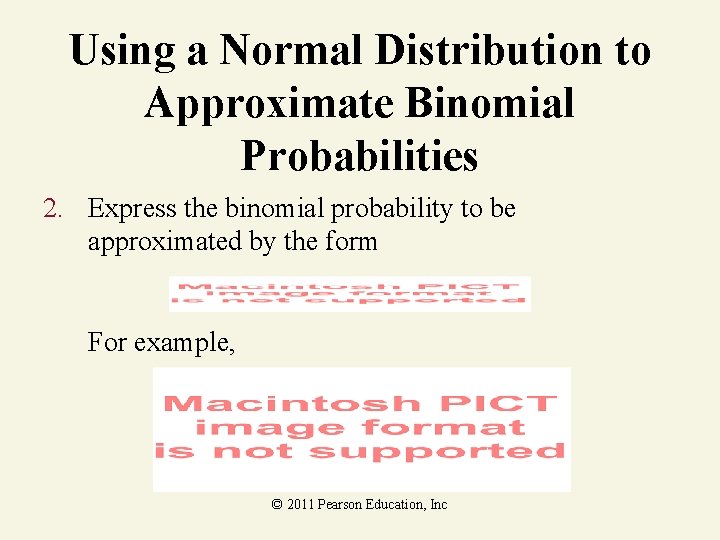
Using a Normal Distribution to Approximate Binomial Probabilities 2. Express the binomial probability to be approximated by the form For example, © 2011 Pearson Education, Inc
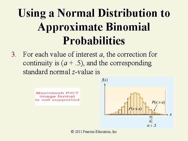
Using a Normal Distribution to Approximate Binomial Probabilities 3. For each value of interest a, the correction for continuity is (a +. 5), and the corresponding standard normal z-value is © 2011 Pearson Education, Inc
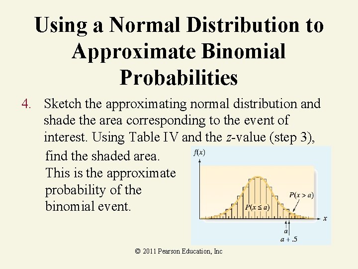
Using a Normal Distribution to Approximate Binomial Probabilities 4. Sketch the approximating normal distribution and shade the area corresponding to the event of interest. Using Table IV and the z-value (step 3), find the shaded area. This is the approximate probability of the binomial event. © 2011 Pearson Education, Inc
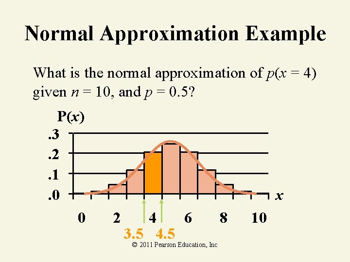
Normal Approximation Example What is the normal approximation of p(x = 4) given n = 10, and p = 0. 5? P(x). 3. 2. 1. 0 0 x 2 4 6 3. 5 4. 5 © 2011 Pearson Education, Inc 8 10
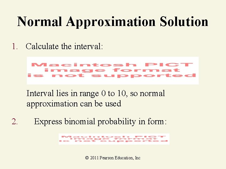
Normal Approximation Solution 1. Calculate the interval: Interval lies in range 0 to 10, so normal approximation can be used 2. Express binomial probability in form: © 2011 Pearson Education, Inc
Normal Approximation Solution 3. Compute standard normal z values: © 2011 Pearson Education, Inc
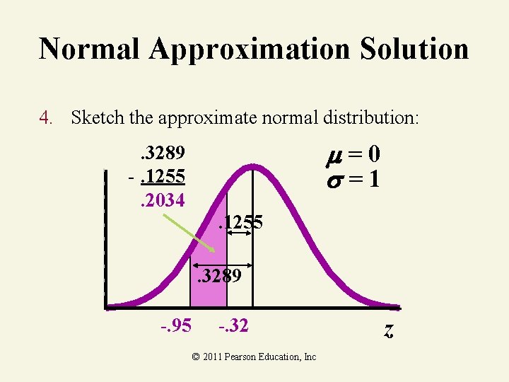
Normal Approximation Solution 4. Sketch the approximate normal distribution: =0 =1 . 3289 -. 1255. 2034. 1255. 3289 -. 95 -. 32 © 2011 Pearson Education, Inc z
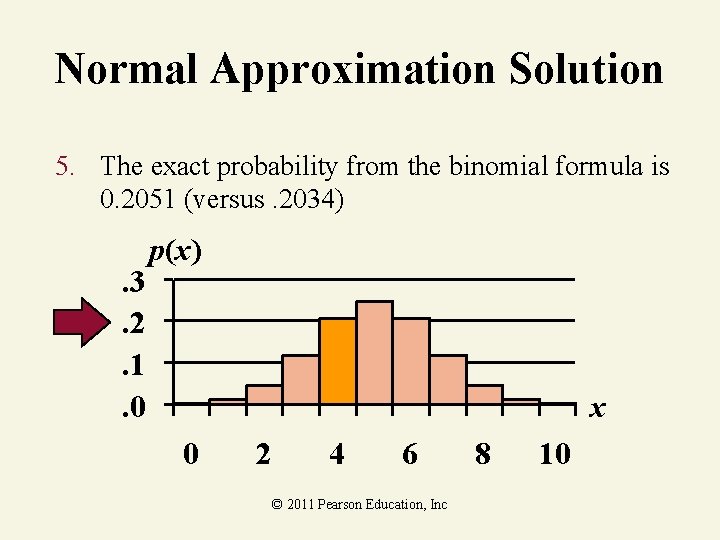
Normal Approximation Solution 5. The exact probability from the binomial formula is 0. 2051 (versus. 2034) . 3. 2. 1. 0 p(x) x 0 2 4 6 © 2011 Pearson Education, Inc 8 10
4. 9 Other Continuous Distributions: Uniform and Exponential © 2011 Pearson Education, Inc
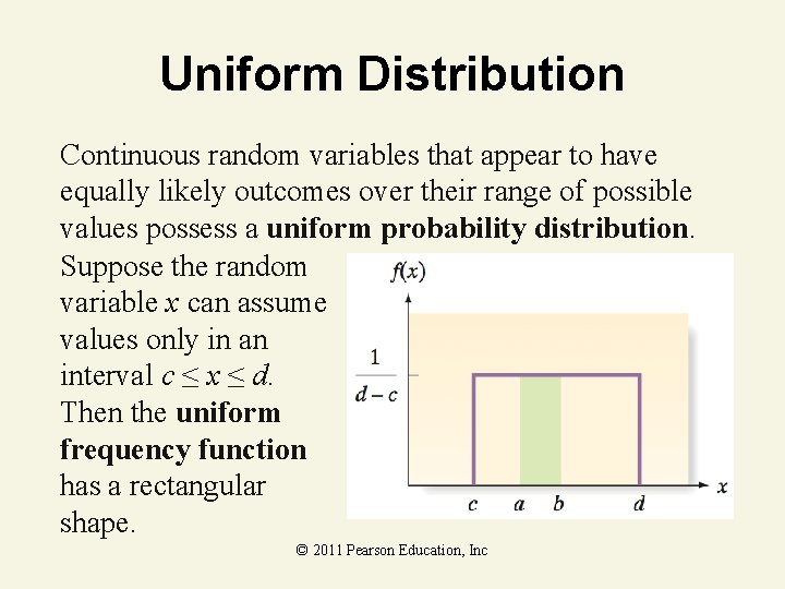
Uniform Distribution Continuous random variables that appear to have equally likely outcomes over their range of possible values possess a uniform probability distribution. Suppose the random variable x can assume values only in an interval c ≤ x ≤ d. Then the uniform frequency function has a rectangular shape. © 2011 Pearson Education, Inc
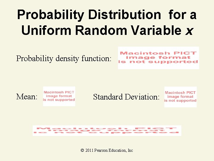
Probability Distribution for a Uniform Random Variable x Probability density function: Mean: Standard Deviation: © 2011 Pearson Education, Inc
Uniform Distribution Example You’re production manager of a soft drink bottling company. You believe that when a machine is set to dispense 12 oz. , it really dispenses between 11. 5 and 12. 5 oz. inclusive. Suppose the amount dispensed has a uniform distribution. What is the probability that less than 11. 8 oz. is dispensed? © 2011 Pearson Education, Inc SODA
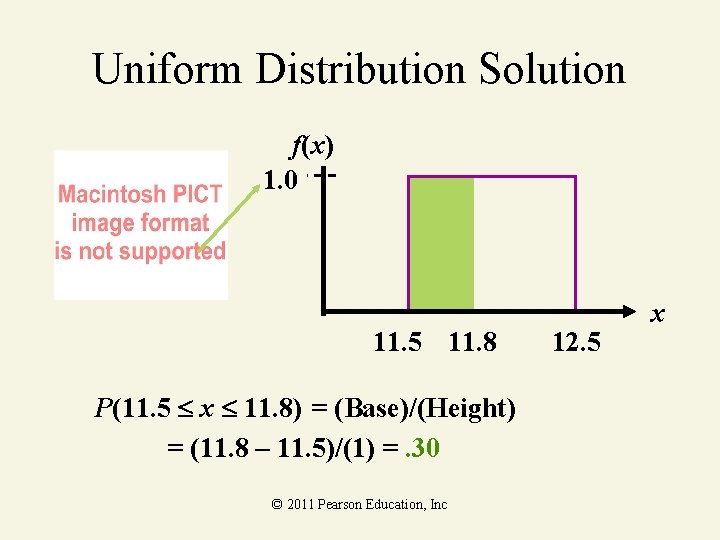
Uniform Distribution Solution f(x) 1. 0 11. 5 11. 8 P(11. 5 x 11. 8) = (Base)/(Height) = (11. 8 – 11. 5)/(1) =. 30 © 2011 Pearson Education, Inc 12. 5 x
Exponential Distribution The length of time between emergency arrivals at a hospital, the length of time between breakdowns of manufacturing equipment, and the length of time between catastrophic events (e. g. , a stockmarket crash), are all continuous random phenomena that we might want to describe probabilistically. The length of time or the distance between occurrences of random events like these can often be described by the exponential probability distribution. For this reason, the exponential distribution is sometimes called the waiting-time distribution. © 2011 Pearson Education, Inc
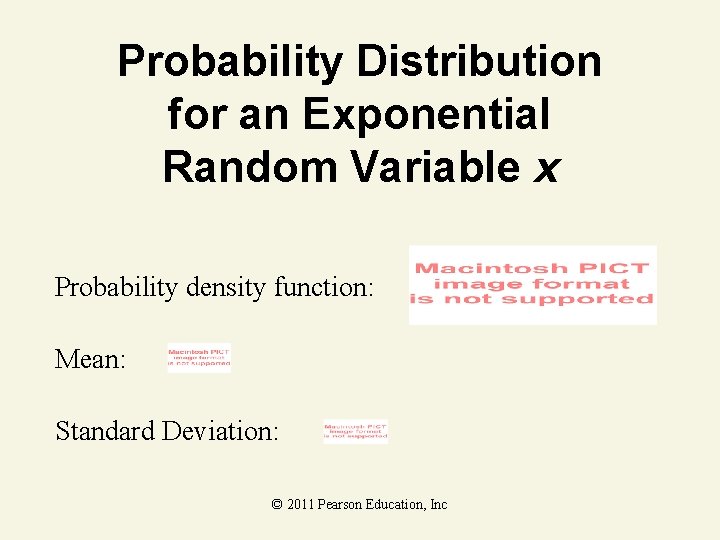
Probability Distribution for an Exponential Random Variable x Probability density function: Mean: Standard Deviation: © 2011 Pearson Education, Inc
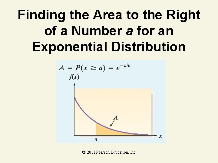
Finding the Area to the Right of a Number a for an Exponential Distribution © 2011 Pearson Education, Inc
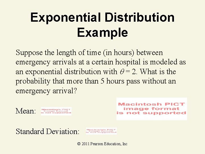
Exponential Distribution Example Suppose the length of time (in hours) between emergency arrivals at a certain hospital is modeled as an exponential distribution with = 2. What is the probability that more than 5 hours pass without an emergency arrival? Mean: Standard Deviation: © 2011 Pearson Education, Inc
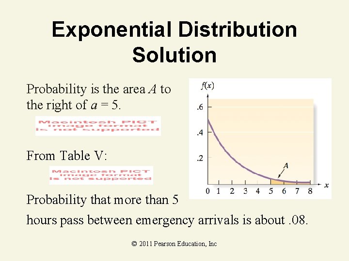
Exponential Distribution Solution Probability is the area A to the right of a = 5. From Table V: Probability that more than 5 hours pass between emergency arrivals is about. 08. © 2011 Pearson Education, Inc
4. 10 Sampling Distributions © 2011 Pearson Education, Inc
Parameter & Statistic A parameter is a numerical descriptive measure of a population. Because it is based on all the observations in the population, its value is almost always unknown. A sample statistic is a numerical descriptive measure of a sample. It is calculated from the observations in the sample. © 2011 Pearson Education, Inc
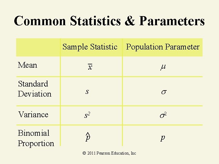
Common Statistics & Parameters Sample Statistic Population Parameter Mean x Standard Deviation s Variance s 2 Binomial Proportion ^ p p © 2011 Pearson Education, Inc
Sampling Distribution The sampling distribution of a sample statistic calculated from a sample of n measurements is the probability distribution of the statistic. © 2011 Pearson Education, Inc
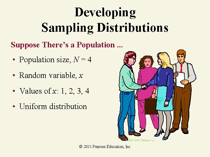
Developing Sampling Distributions Suppose There’s a Population. . . • Population size, N = 4 • Random variable, x • Values of x: 1, 2, 3, 4 • Uniform distribution © 1984 -1994 T/Maker Co. © 2011 Pearson Education, Inc
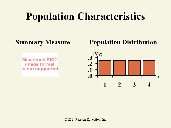
Population Characteristics Summary Measure Population Distribution. 3. 2. 1. 0 P(x) x 1 © 2011 Pearson Education, Inc 2 3 4
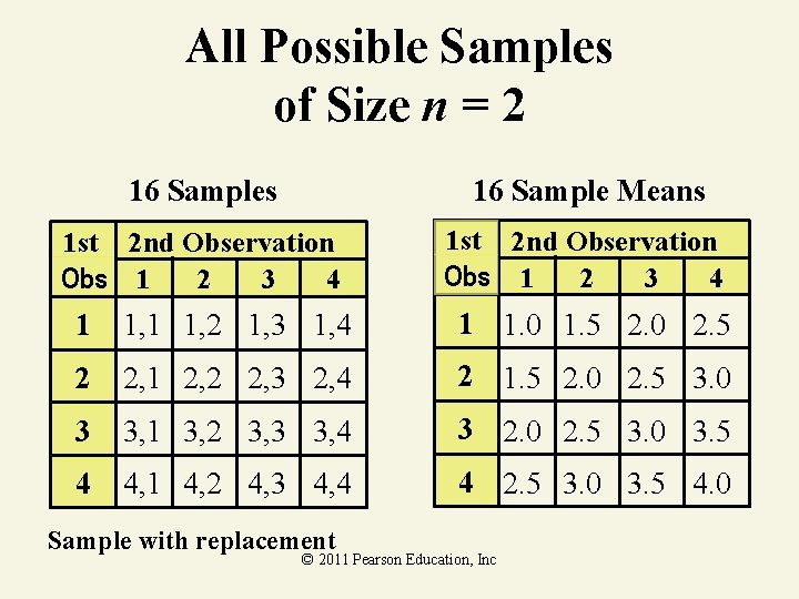
All Possible Samples of Size n = 2 16 Samples 16 Sample Means 1 st 2 nd Observation Obs 1 2 3 4 1 1, 2 1, 3 1, 4 1 1. 0 1. 5 2. 0 2. 5 2 2, 1 2, 2 2, 3 2, 4 2 1. 5 2. 0 2. 5 3. 0 3 3, 1 3, 2 3, 3 3, 4 3 2. 0 2. 5 3. 0 3. 5 4 4, 1 4, 2 4, 3 4, 4 4 2. 5 3. 0 3. 5 4. 0 Sample with replacement © 2011 Pearson Education, Inc
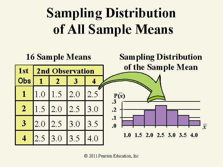
Sampling Distribution of All Sample Means 16 Sample Means 1 st 2 nd Observation Obs 1 2 3 4 1 1. 0 1. 5 2. 0 2. 5 2 1. 5 2. 0 2. 5 3. 0 3. 5 4. 0 Sampling Distribution of the Sample Mean P(x). 3. 2. 1. 0 1. 5 2. 0 2. 5 3. 0 3. 5 4. 0 © 2011 Pearson Education, Inc x
Summary Measure of All Sample Means © 2011 Pearson Education, Inc
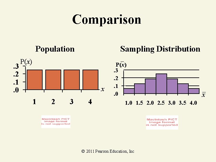
Comparison Population. 3. 2. 1. 0 Sampling Distribution P(x) x 1 2 3 4 P(x). 3. 2. 1. 0 1. 5 2. 0 2. 5 3. 0 3. 5 4. 0 © 2011 Pearson Education, Inc x
4. 11 The Sampling Distribution of a Sample Mean and the Central Limit Theorem © 2011 Pearson Education, Inc
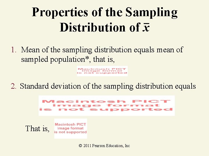
Properties of the Sampling Distribution of x 1. Mean of the sampling distribution equals mean of sampled population*, that is, 2. Standard deviation of the sampling distribution equals That is, © 2011 Pearson Education, Inc
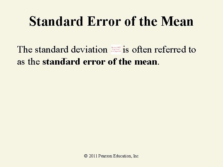
Standard Error of the Mean The standard deviation is often referred to as the standard error of the mean. © 2011 Pearson Education, Inc
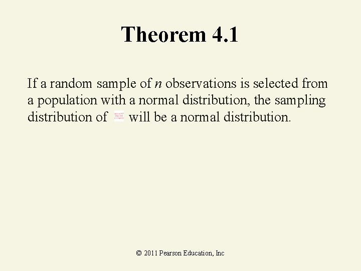
Theorem 4. 1 If a random sample of n observations is selected from a population with a normal distribution, the sampling distribution of will be a normal distribution. © 2011 Pearson Education, Inc
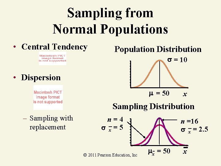
Sampling from Normal Populations • Central Tendency Population Distribution = 10 • Dispersion m = 50 x Sampling Distribution – Sampling with replacement n=4 x = 5 © 2011 Pearson Education, Inc n =16 x = 2. 5 mx- = 50 x
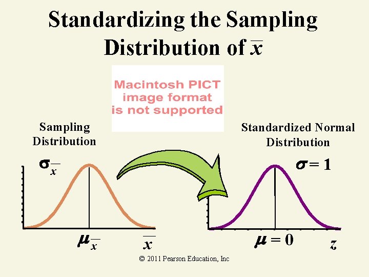
Standardizing the Sampling Distribution of x Sampling Distribution Standardized Normal Distribution = 1 x x x © 2011 Pearson Education, Inc =0 z
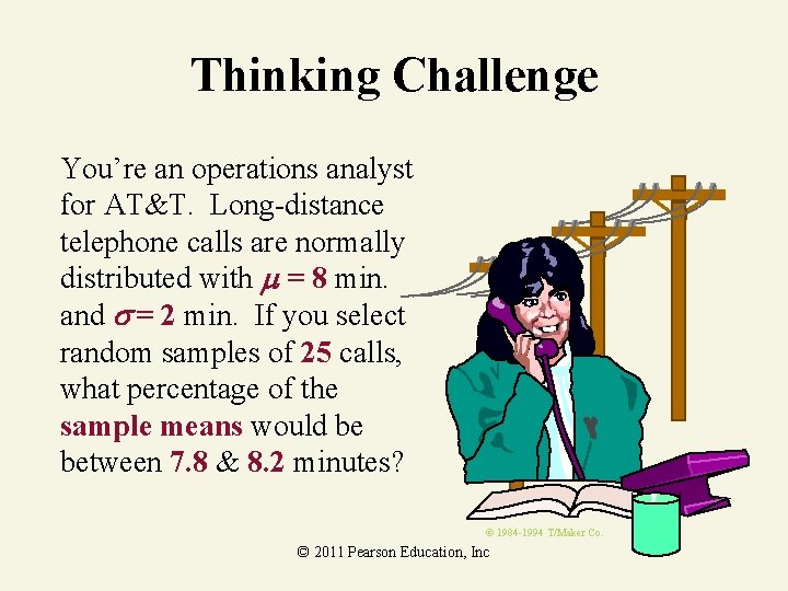
Thinking Challenge You’re an operations analyst for AT&T. Long-distance telephone calls are normally distributed with = 8 min. and = 2 min. If you select random samples of 25 calls, what percentage of the sample means would be between 7. 8 & 8. 2 minutes? © 1984 -1994 T/Maker Co. © 2011 Pearson Education, Inc
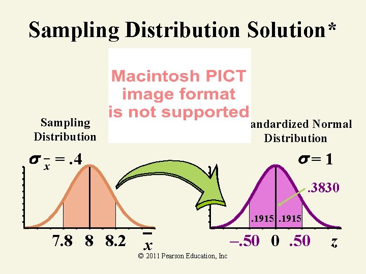
Sampling Distribution Solution* Sampling Distribution x =. 4 Standardized Normal Distribution =1. 3830. 1915 7. 8 8 8. 2 x –. 50 0. 50 © 2011 Pearson Education, Inc z
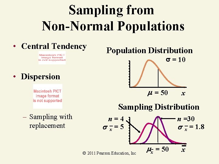
Sampling from Non-Normal Populations • Central Tendency Population Distribution = 10 • Dispersion = 50 x Sampling Distribution – Sampling with replacement n=4 x = 5 © 2011 Pearson Education, Inc n =30 x = 1. 8 x- = 50 x
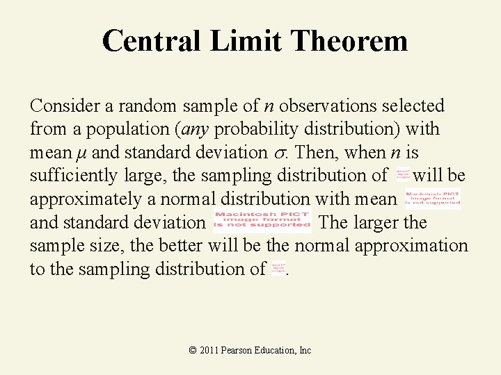
Central Limit Theorem Consider a random sample of n observations selected from a population (any probability distribution) with mean μ and standard deviation . Then, when n is sufficiently large, the sampling distribution of will be approximately a normal distribution with mean and standard deviation The larger the sample size, the better will be the normal approximation to the sampling distribution of. © 2011 Pearson Education, Inc
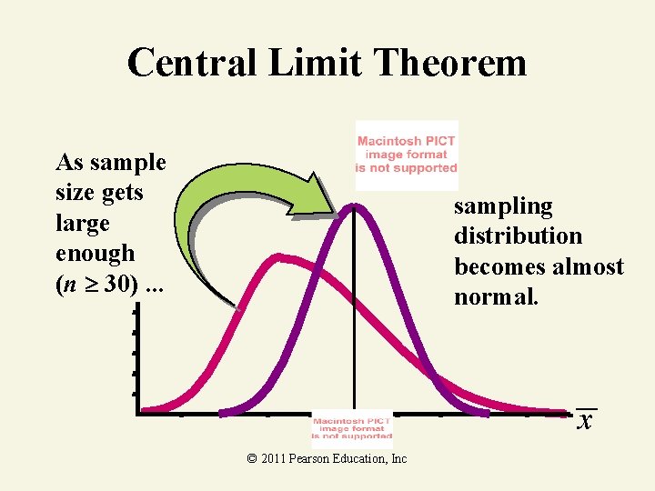
Central Limit Theorem As sample size gets large enough (n 30). . . sampling distribution becomes almost normal. x © 2011 Pearson Education, Inc
Central Limit Theorem Example The amount of soda in cans of a particular brand has a mean of 12 oz and a standard deviation of. 2 oz. If you select random samples of 50 cans, what percentage of the sample means would be less than 11. 95 oz? © 2011 Pearson Education, Inc SODA
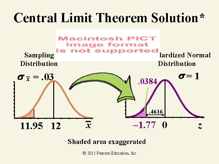
Central Limit Theorem Solution* Sampling Distribution Standardized Normal Distribution x =. 0384 =1 . 4616 11. 95 12 x – 1. 77 0 Shaded area exaggerated © 2011 Pearson Education, Inc z
Key Ideas Properties of Probability Distributions Discrete Distributions 1. p(x) ≥ 0 2. Continuous Distributions 1. P(x = a) = 0 2. P(a < x < b) = area under curve between a and b © 2011 Pearson Education, Inc
Key Ideas Normal Approximation to Binomial x is binomial (n, p) © 2011 Pearson Education, Inc
Key Ideas Methods for Assessing Normality 1. Histogram © 2011 Pearson Education, Inc
Key Ideas Methods for Assessing Normality 2. Stem-and-leaf display 1 7 2 3389 3 245677 4 19 5 2 © 2011 Pearson Education, Inc
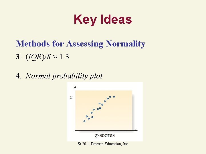
Key Ideas Methods for Assessing Normality 3. (IQR)/S ≈ 1. 3 4. Normal probability plot © 2011 Pearson Education, Inc
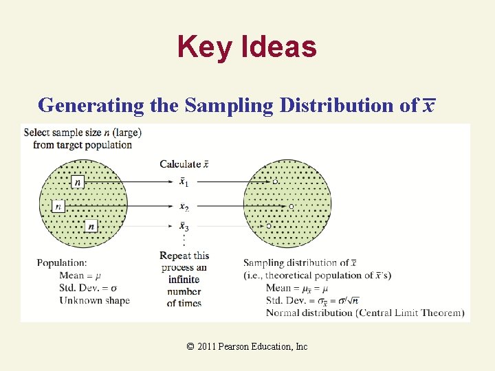
Key Ideas Generating the Sampling Distribution of x © 2011 Pearson Education, Inc
- Slides: 132