2 The Rectangular Coordinate System and Graphs of

2 The Rectangular Coordinate System and Graphs of Equations

Chapter Overview Mathematical expressions often indicate relationships between two variables. • To visualize these relationships, we draw graphs of their equations.

2. 1 The Rectangular Coordinate System

Objectives 1. Plot Points in the Rectangular Coordinate System 2. Graph Linear Equations 3. Graph Horizontal and Vertical Lines 4. Solve Problems Using Linear Equations 5. Find the Distance Between Two Points 6. Find the Midpoint of a Line Segment

Solutions of an Equation The solutions of an equation with variables x and y such as y = – 1/2 x + 4 are ordered pairs of real numbers (x, y) that satisfy the equation. • To find some ordered pairs that satisfy the equation, we substitute input values of x into the equation and find the corresponding output values of y.

Solutions of an Equation For example, if we substitute 2 for x, we obtain y = 3. • Since y = 3 when x = 2, the ordered pair (2, 3) is a solution of the equation. • The first coordinate, 2, of the ordered pair is usually called the x-coordinate. • The second coordinate, 3, is usually called the y-coordinate.

1. Plot Points in the Rectangular Coordinate System

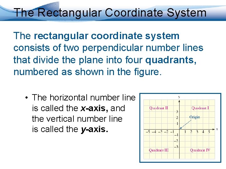
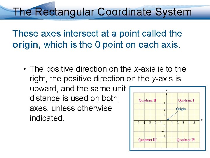
The Rectangular Coordinate System The rectangular coordinate system consists of two perpendicular number lines that divide the plane into four quadrants, numbered as shown in the figure. • The horizontal number line is called the x-axis, and the vertical number line is called the y-axis.

The Rectangular Coordinate System These axes intersect at a point called the origin, which is the 0 point on each axis. • The positive direction on the x-axis is to the right, the positive direction on the y-axis is upward, and the same unit distance is used on both axes, unless otherwise indicated.

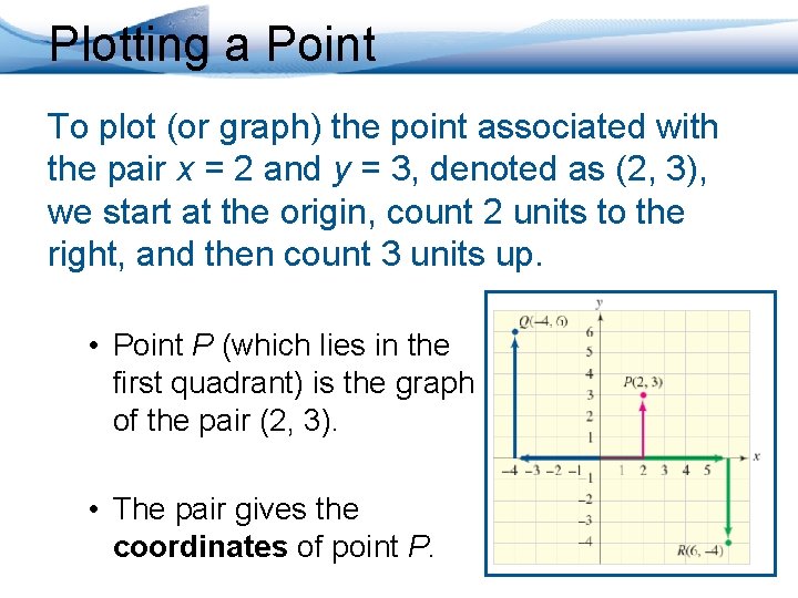
Plotting a Point To plot (or graph) the point associated with the pair x = 2 and y = 3, denoted as (2, 3), we start at the origin, count 2 units to the right, and then count 3 units up. • Point P (which lies in the first quadrant) is the graph of the pair (2, 3). • The pair gives the coordinates of point P.

2. Graph Linear Equations

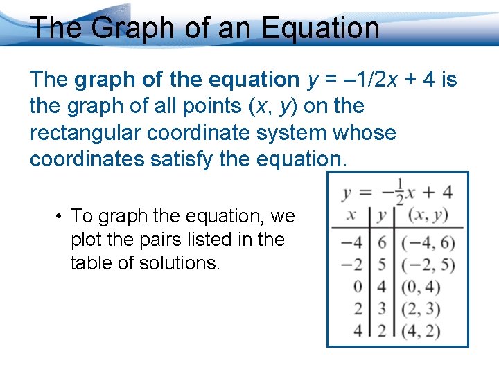
The Graph of an Equation The graph of the equation y = – 1/2 x + 4 is the graph of all points (x, y) on the rectangular coordinate system whose coordinates satisfy the equation. • To graph the equation, we plot the pairs listed in the table of solutions.

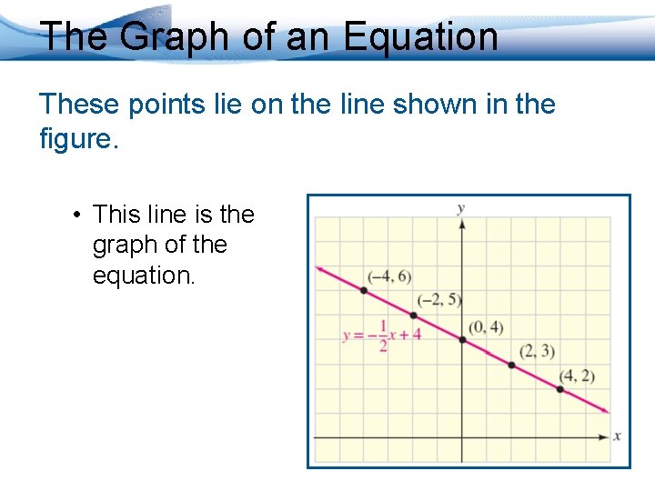
The Graph of an Equation These points lie on the line shown in the figure. • This line is the graph of the equation.

Comment When we say that the graph of an equation is a line, we imply two things: 1. Every point with coordinates that satisfy the equation will lie on the line. 2. Every point on the line will have coordinates that satisfy the equation.

Linear Equations When the graph of an equation is a line, we call the equation a linear equation. • These equations often are written in standard form as Ax + By = C, where A, B and C are specific numbers (called constants) and x and y are variables. • Either A or B can be 0, but A and B cannot both be 0.

Intercepts of a Line The y-intercept of a line is the point (0, b), where the line intersects the y-axis. • To find b, substitute 0 for x in the equation of the line and solve for y. The x-intercept of a line is the point (a, 0), where the line intersects the x-axis. • To find a, substitute 0 for y in the equation of the line and solve for x.

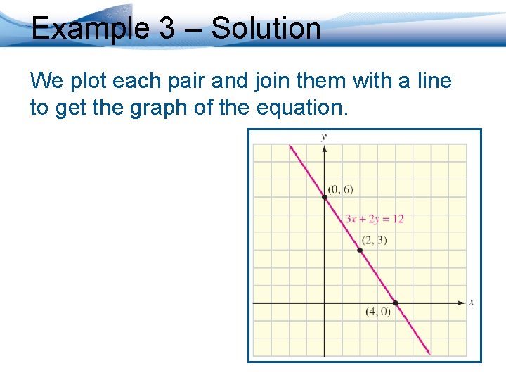
Example 3 Use the x- and y-intercepts to graph the equation 3 x + 2 y = 12. • To find the intercepts, we will use the method described earlier. • We will also find a third point as a check and then plot the points and draw the graph.

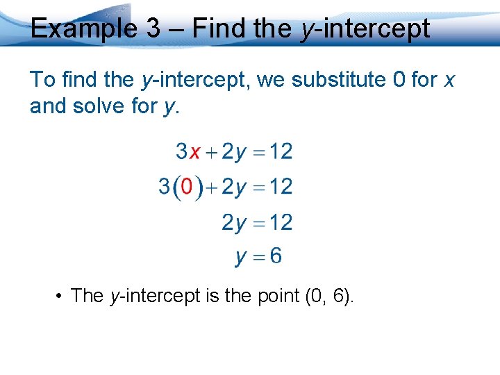
Example 3 – Find the y-intercept To find the y-intercept, we substitute 0 for x and solve for y. • The y-intercept is the point (0, 6).

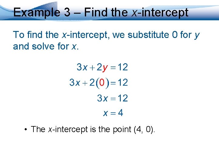
Example 3 – Find the x-intercept To find the x-intercept, we substitute 0 for y and solve for x. • The x-intercept is the point (4, 0).

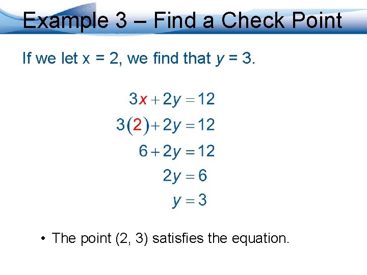
Example 3 – Find a Check Point If we let x = 2, we find that y = 3. • The point (2, 3) satisfies the equation.

Example 3 – Solution We plot each pair and join them with a line to get the graph of the equation.

3. Graph Horizontal and Vertical Lines

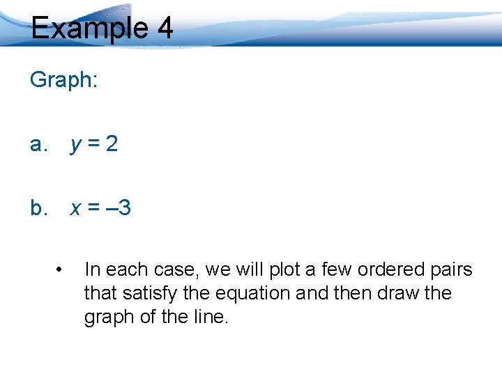
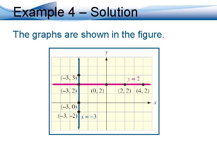
Example 4 Graph: a. y = 2 b. x = – 3 • In each case, we will plot a few ordered pairs that satisfy the equation and then draw the graph of the line.

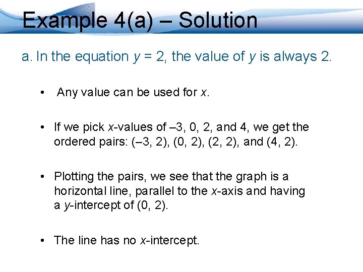
Example 4(a) – Solution a. In the equation y = 2, the value of y is always 2. • Any value can be used for x. • If we pick x-values of – 3, 0, 2, and 4, we get the ordered pairs: (– 3, 2), (0, 2), (2, 2), and (4, 2). • Plotting the pairs, we see that the graph is a horizontal line, parallel to the x-axis and having a y-intercept of (0, 2). • The line has no x-intercept.

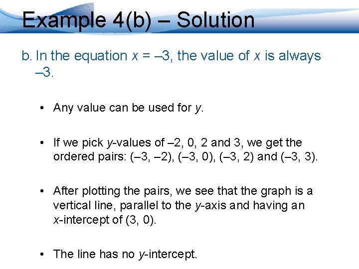
Example 4(b) – Solution b. In the equation x = – 3, the value of x is always – 3. • Any value can be used for y. • If we pick y-values of – 2, 0, 2 and 3, we get the ordered pairs: (– 3, – 2), (– 3, 0), (– 3, 2) and (– 3, 3). • After plotting the pairs, we see that the graph is a vertical line, parallel to the y-axis and having an x-intercept of (3, 0). • The line has no y-intercept.

Example 4 – Solution The graphs are shown in the figure.

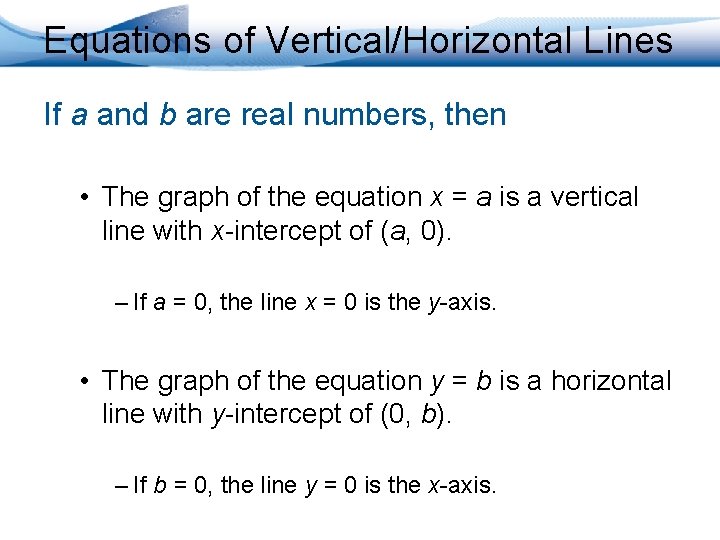
Equations of Vertical/Horizontal Lines If a and b are real numbers, then • The graph of the equation x = a is a vertical line with x-intercept of (a, 0). – If a = 0, the line x = 0 is the y-axis. • The graph of the equation y = b is a horizontal line with y-intercept of (0, b). – If b = 0, the line y = 0 is the x-axis.

4. Solve Problems Using Linear Equations

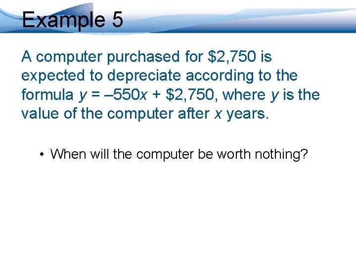
Example 5 A computer purchased for $2, 750 is expected to depreciate according to the formula y = – 550 x + $2, 750, where y is the value of the computer after x years. • When will the computer be worth nothing?

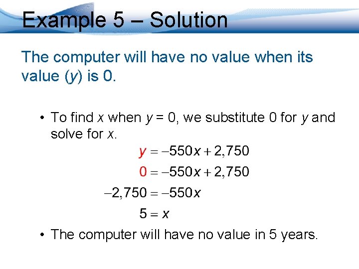
Example 5 – Solution The computer will have no value when its value (y) is 0. • To find x when y = 0, we substitute 0 for y and solve for x. • The computer will have no value in 5 years.

5. Find the Distance between Two Points

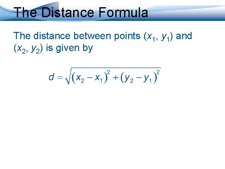
The Distance Formula The distance between points (x 1, y 1) and (x 2, y 2) is given by

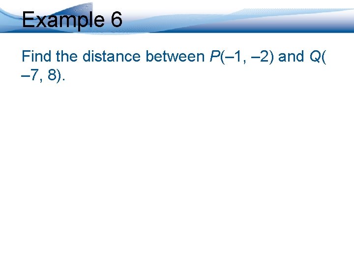
Example 6 Find the distance between P(– 1, – 2) and Q( – 7, 8).

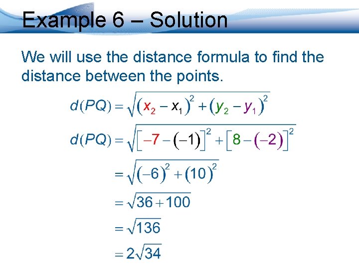
Example 6 – Solution We will use the distance formula to find the distance between the points.

6. Find the Midpoint of a Line Segment

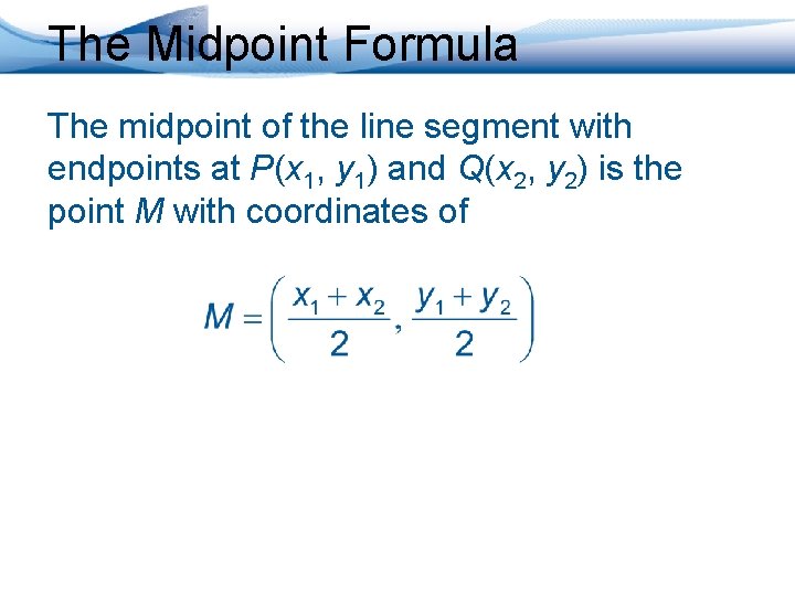
The Midpoint Formula The midpoint of the line segment with endpoints at P(x 1, y 1) and Q(x 2, y 2) is the point M with coordinates of

Example 7 Find the midpoint of the segment joining P(– 7, 2) and Q(1, – 4).

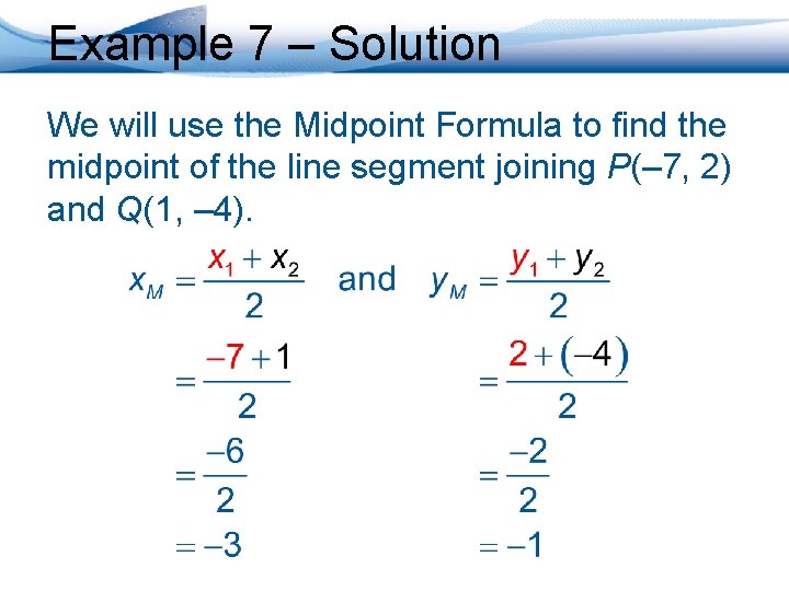
Example 7 – Solution We will use the Midpoint Formula to find the midpoint of the line segment joining P(– 7, 2) and Q(1, – 4).

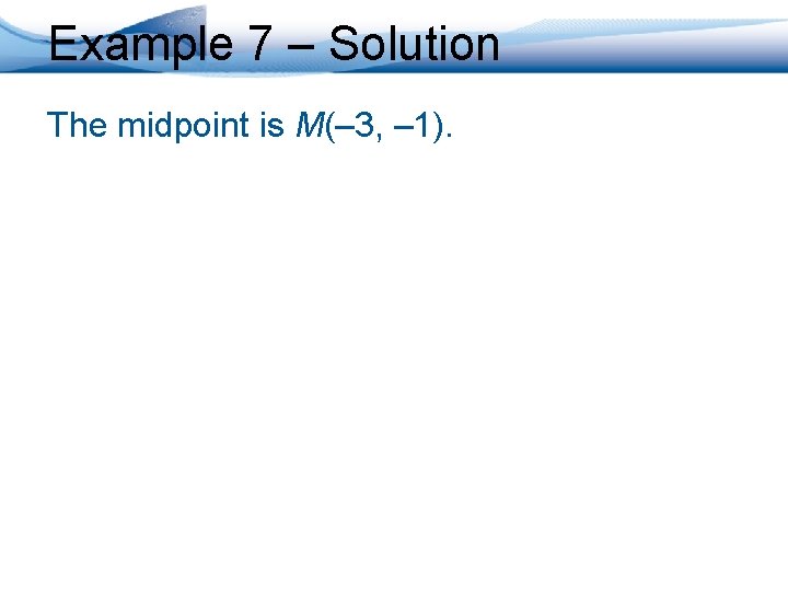
Example 7 – Solution The midpoint is M(– 3, – 1).