2 Structure of electrified interface 1 The electrical

2 Structure of electrified interface 1. The electrical double layer 2. The Gibbs adsorption isotherm 3. Electrocapillary equation 4. Electrosorption phenomena 5. Electrical model of the interface

2. 1 The electrical double layer Historical milestones -The concept electrical double layer Quincke – 1862 -Concept of two parallel layers of opposite charges Helmholtz 1879 and Stern 1924 -Concept of diffuse layer Gouy 1910; Chapman 1913 - Modern model Grahame 1947

Presently accepted model of the electrical double layer

2. 2 Gibbs adsorption isotherm Definitions a s G – total Gibbs function of the system Ga, Gb, Gs - Gibbs functions of phases a, b, s Gibbs function of the surface phase s: b Gs = G – { G a + Gb }

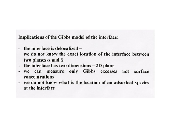
Gibbs Model of the interface

The amount of species j in the surface phase: njs = nj – { nja + njb} Gibbs surface excess Gj Gj = njs/A A – surface area

Gibbs adsorption isotherm Change in G brought about by changes in T, p, A and nj d. G=-Sd. T + Vdp + gd. A + Smjdnj – surface energy – work needed to create a unit area by cleavage - chemical potential d. Ga =-Sad. T + Vadp + + Smjdnja d. Gb =-Sbd. T + Vbdp + + Smjdnjb and d. Gs = d. G – {d. Ga + d. Gb}= Ssd. T + gd. A + + Smjdnjs

Derivation of the Gibbs adsorption isotherm d. Gs = -Ssd. T + gd. A + + Smjdnjs Integrate this expression at costant T and p Gs = Ag + Smjnjs Differentiate Gs d. Gs = Adg + gd. A + Snjsdmj + Smjdnjs The first and the last equations are valid if: Adg + Snjsdmj = 0 or dg = - Gjdmj

Gibbs model of the interface - Summary

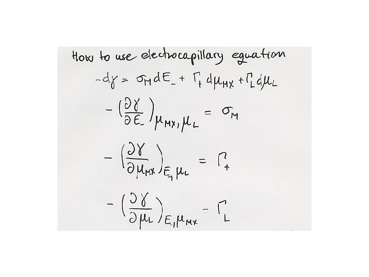
2. 3 The electrocapillary equation Cu’ Ag Ag. Cl KCl, H 2 O, L Hg Cu’’

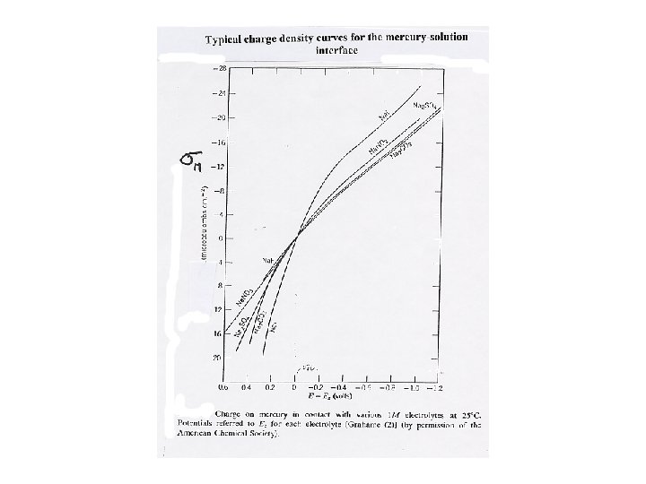
s. M = F(GHg+ - Ge)

Lippmann equation

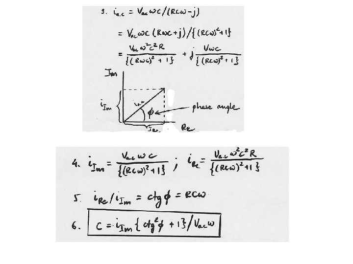
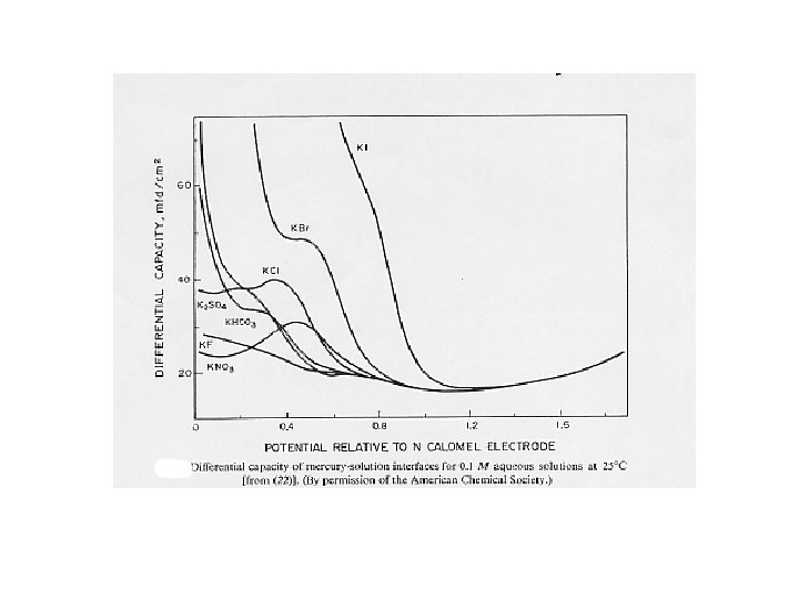
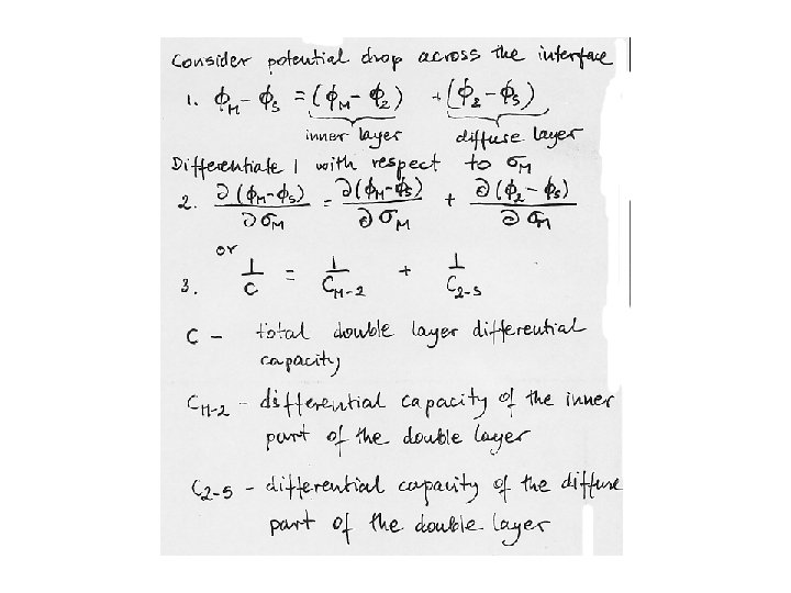
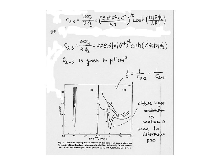
Differential capacity of the interface

Capacity of the diffuse layer Thickness of the diffuse layer

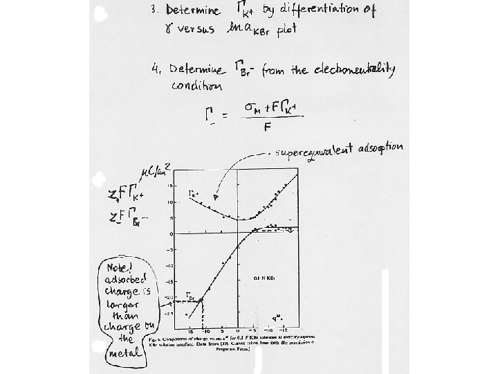
2. 4 Electrosorption phenomena

2. 5 Electrical properties of the interface In the most simple case – ideally polarizable electrode the electrochemical cell can be represented by a simple RC circuit

Implication – electrochemical cell has a time constant that imposes restriction on investigations of fast electrode process Time needed for the potential across the interface to reach The applied value : Ec - potential across the interface E - potential applied from an external generator

Time constant of the cell t = Ru Cd Typical values Ru=50 W; C=2 m. F gives t=100 ms

Current flowing in the absence of a redox reaction – nonfaradaic current In the presence of a redox reaction – faradaic impedance is connected in parallel to the double layer capacitance. The scheme of the cell is: The overall current flowing through the cell is : i = if + inf Only the faradaic current –if contains analytical or kinetic information