2 IV 60 Computer graphics set 9 Splines

2 IV 60 Computer graphics set 9: Splines Jack van Wijk TU/e

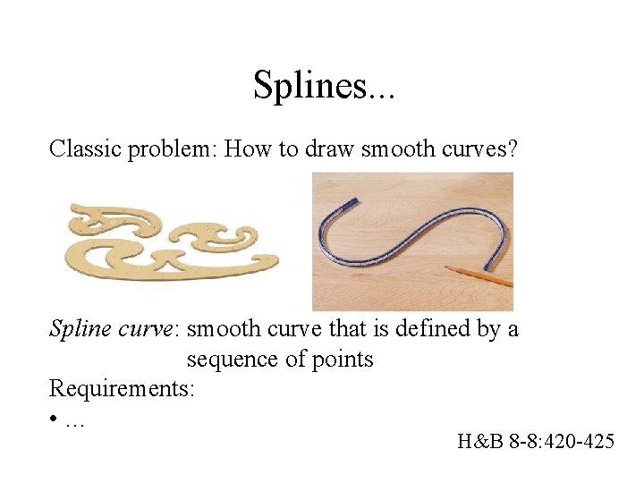
Splines. . . Classic problem: How to draw smooth curves? Spline curve: smooth curve that is defined by a sequence of points Requirements: • … H&B 8 -8: 420 -425

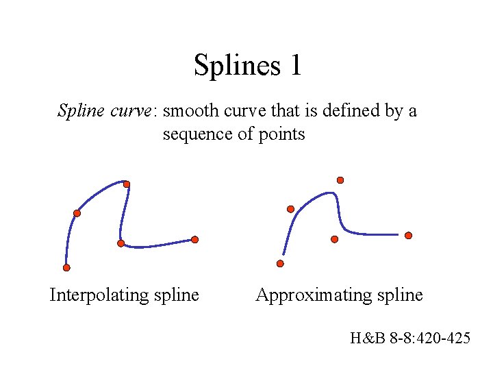
Splines 1 Spline curve: smooth curve that is defined by a sequence of points Interpolating spline Approximating spline H&B 8 -8: 420 -425

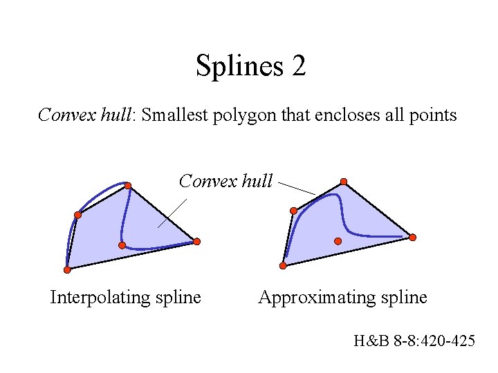
Splines 2 Convex hull: Smallest polygon that encloses all points Convex hull Interpolating spline Approximating spline H&B 8 -8: 420 -425

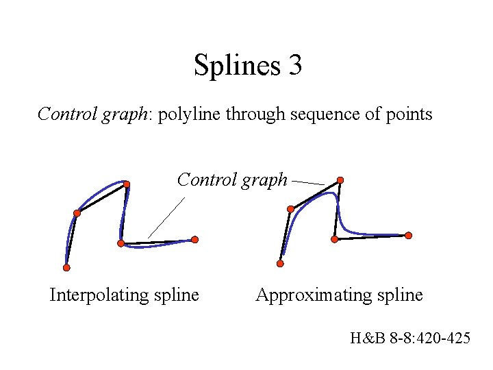
Splines 3 Control graph: polyline through sequence of points Control graph Interpolating spline Approximating spline H&B 8 -8: 420 -425

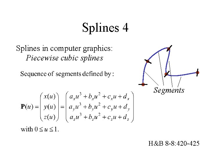
Splines 4 Splines in computer graphics: Piecewise cubic splines Segments H&B 8 -8: 420 -425

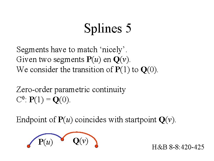
Splines 5 Segments have to match ‘nicely’. Given two segments P(u) en Q(v). We consider the transition of P(1) to Q(0). Zero-order parametric continuity C 0: P(1) = Q(0). Endpoint of P(u) coincides with startpoint Q(v). P(u) Q(v) H&B 8 -8: 420 -425

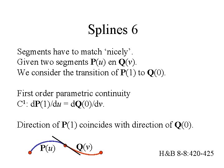
Splines 6 Segments have to match ‘nicely’. Given two segments P(u) en Q(v). We consider the transition of P(1) to Q(0). First order parametric continuity C 1: d. P(1)/du = d. Q(0)/dv. Direction of P(1) coincides with direction of Q(0). P(u) Q(v) H&B 8 -8: 420 -425

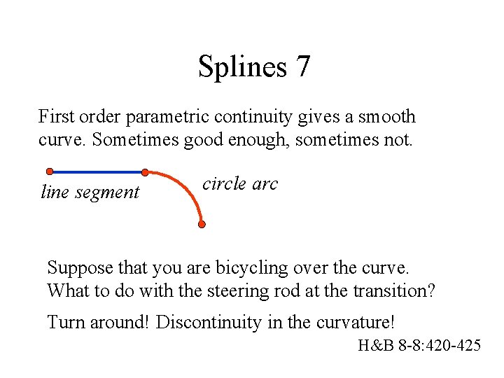
Splines 7 First order parametric continuity gives a smooth curve. Sometimes good enough, sometimes not. line segment circle arc Suppose that you are bicycling over the curve. What to do with the steering rod at the transition? Turn around! Discontinuity in the curvature! H&B 8 -8: 420 -425

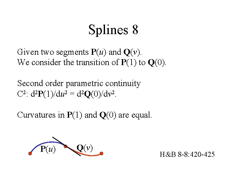
Splines 8 Given two segments P(u) and Q(v). We consider the transition of P(1) to Q(0). Second order parametric continuity C 2: d 2 P(1)/du 2 = d 2 Q(0)/dv 2. Curvatures in P(1) and Q(0) are equal. P(u) Q(v) H&B 8 -8: 420 -425

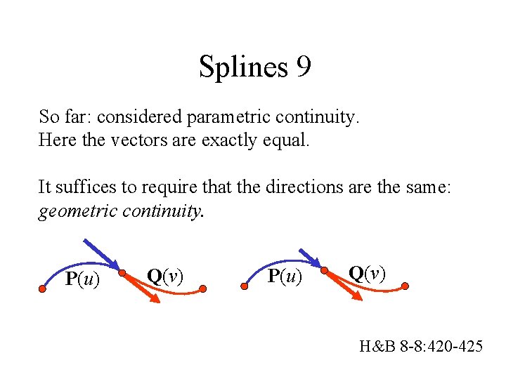
Splines 9 So far: considered parametric continuity. Here the vectors are exactly equal. It suffices to require that the directions are the same: geometric continuity. P(u) Q(v) H&B 8 -8: 420 -425

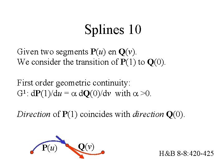
Splines 10 Given two segments P(u) en Q(v). We consider the transition of P(1) to Q(0). First order geometric continuity: G 1: d. P(1)/du = d. Q(0)/dv with >0. Direction of P(1) coincides with direction Q(0). P(u) Q(v) H&B 8 -8: 420 -425

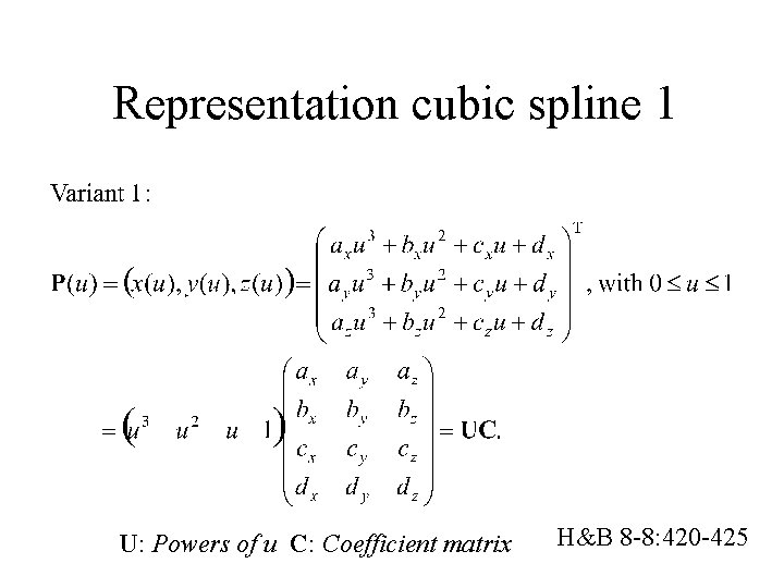
Representation cubic spline 1 U: Powers of u C: Coefficient matrix H&B 8 -8: 420 -425

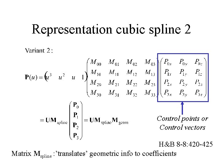
Representation cubic spline 2 Control points or Control vectors H&B 8 -8: 420 -425 Matrix Mspline : ’translates’ geometric info to coefficients

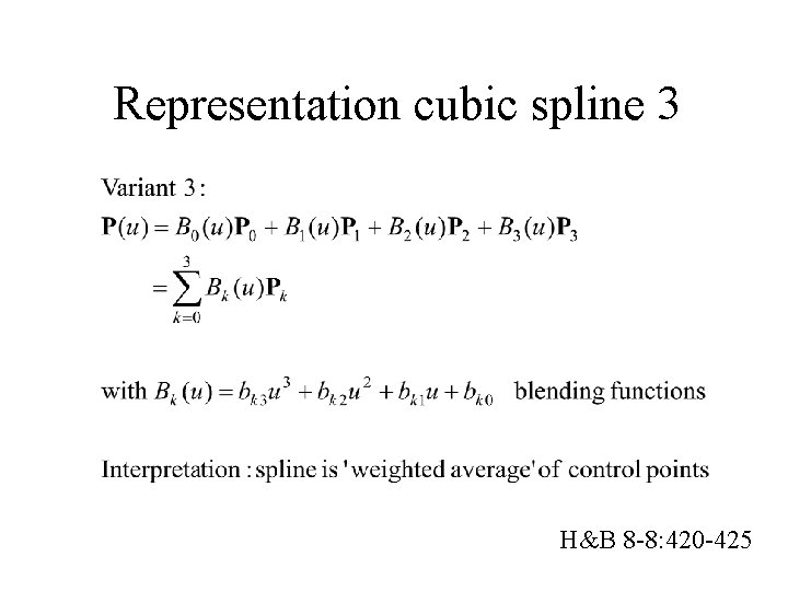
Representation cubic spline 3 H&B 8 -8: 420 -425

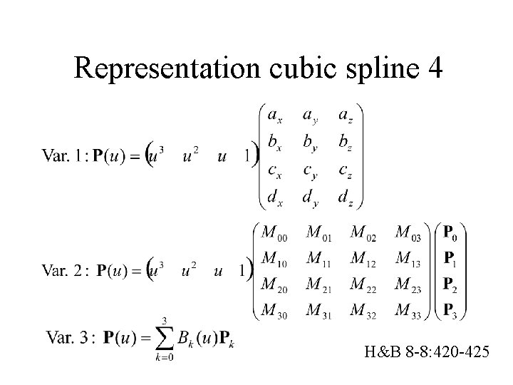
Representation cubic spline 4 H&B 8 -8: 420 -425

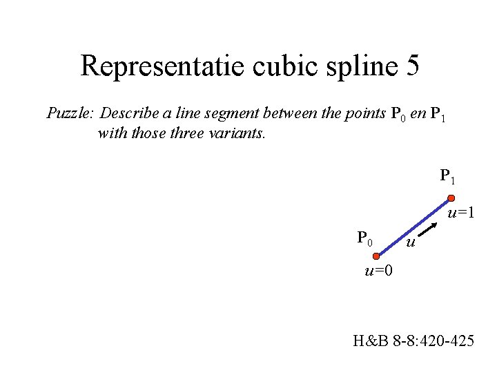
Representatie cubic spline 5 Puzzle: Describe a line segment between the points P 0 en P 1 with those three variants. P 1 u=1 P 0 u u=0 H&B 8 -8: 420 -425

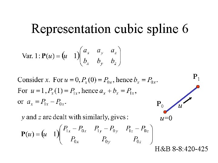
Representation cubic spline 6 P 1 P 0 u u=0 H&B 8 -8: 420 -425

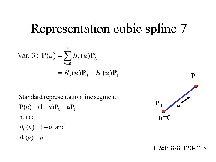
Representation cubic spline 7 P 1 P 0 u u=0 H&B 8 -8: 420 -425

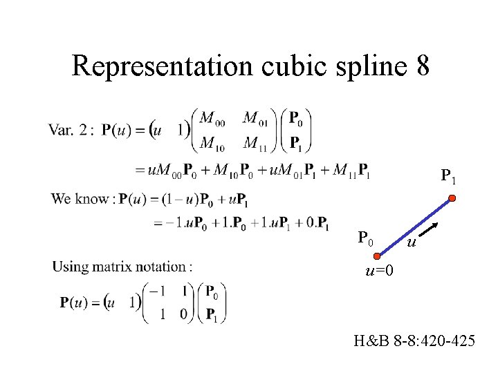
Representation cubic spline 8 P 1 P 0 u u=0 H&B 8 -8: 420 -425

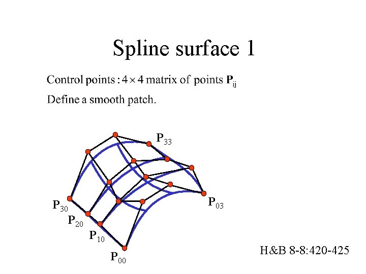
Spline surface 1 P 33 P 30 P 20 P 03 P 10 P 00 H&B 8 -8: 420 -425

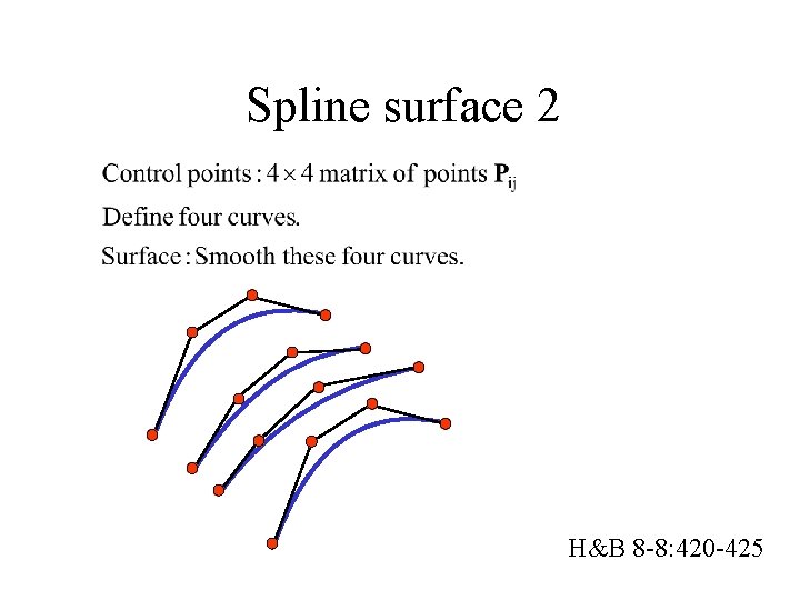
Spline surface 2 H&B 8 -8: 420 -425

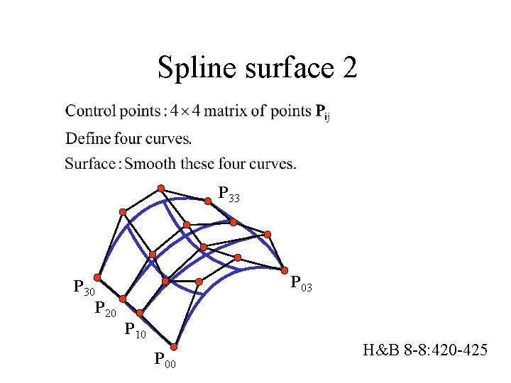
Spline surface 2 P 33 P 30 P 20 P 03 P 10 P 00 H&B 8 -8: 420 -425

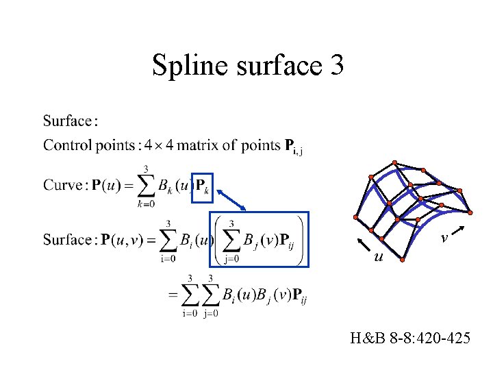
Spline surface 3 v u H&B 8 -8: 420 -425

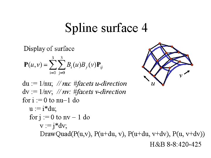
Spline surface 4 v u du : = 1/nu; // nu: #facets u-direction dv : = 1/nv; // nv: #facets v-direction for i : = 0 to nu 1 do u : = i*du; for j : = 0 to nv 1 do v : = j*dv; Draw. Quad(P(u, v), P(u+du, v+dv), P(u, v+dv)) H&B 8 -8: 420 -425

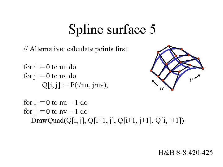
Spline surface 5 // Alternative: calculate points first for i : = 0 to nu do for j : = 0 to nv do Q[i, j] : = P(i/nu, j/nv); v u for i : = 0 to nu 1 do for j : = 0 to nv 1 do Draw. Quad(Q[i, j], Q[i+1, j+1], Q[i, j+1]) H&B 8 -8: 420 -425

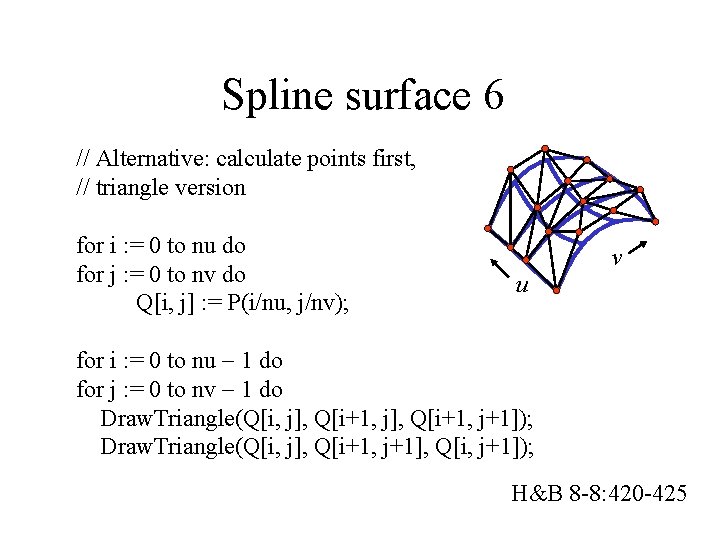
Spline surface 6 // Alternative: calculate points first, // triangle version for i : = 0 to nu do for j : = 0 to nv do Q[i, j] : = P(i/nu, j/nv); v u for i : = 0 to nu 1 do for j : = 0 to nv 1 do Draw. Triangle(Q[i, j], Q[i+1, j+1]); Draw. Triangle(Q[i, j], Q[i+1, j+1], Q[i, j+1]); H&B 8 -8: 420 -425

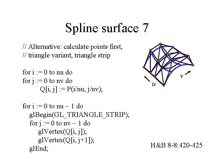
Spline surface 7 // Alternative: calculate points first, // triangle variant, triangle strip for i : = 0 to nu do for j : = 0 to nv do Q[i, j] : = P(i/nu, j/nv); for i : = 0 to nu 1 do gl. Begin(GL_TRIANGLE_STRIP); for j : = 0 to nv 1 do gl. Vertex(Q[i, j]); gl. Vertex(Q[i, j+1]); gl. End; v u H&B 8 -8: 420 -425

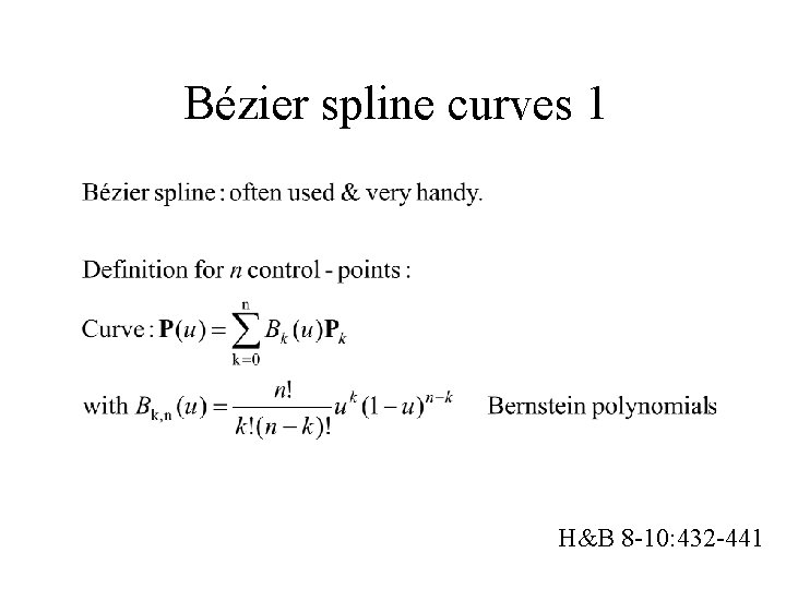
Bézier spline curves 1 H&B 8 -10: 432 -441

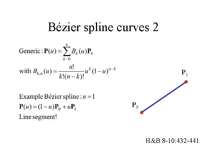
Bézier spline curves 2 P 1 P 0 H&B 8 -10: 432 -441

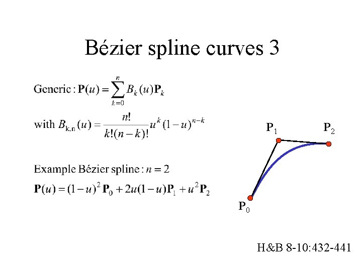
Bézier spline curves 3 P 1 P 2 P 0 H&B 8 -10: 432 -441

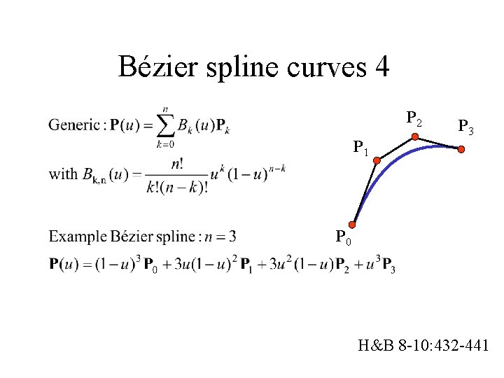
Bézier spline curves 4 P 2 P 1 P 3 P 0 H&B 8 -10: 432 -441

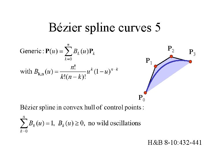
Bézier spline curves 5 P 2 P 1 P 3 P 0 H&B 8 -10: 432 -441

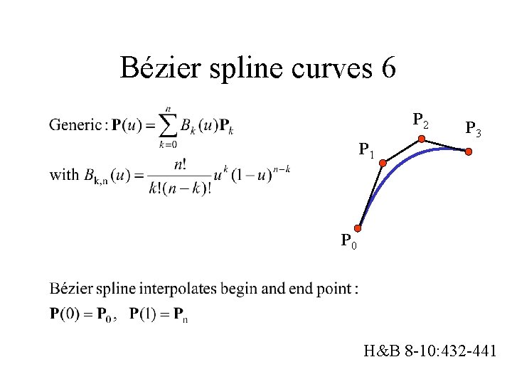
Bézier spline curves 6 P 2 P 1 P 3 P 0 H&B 8 -10: 432 -441

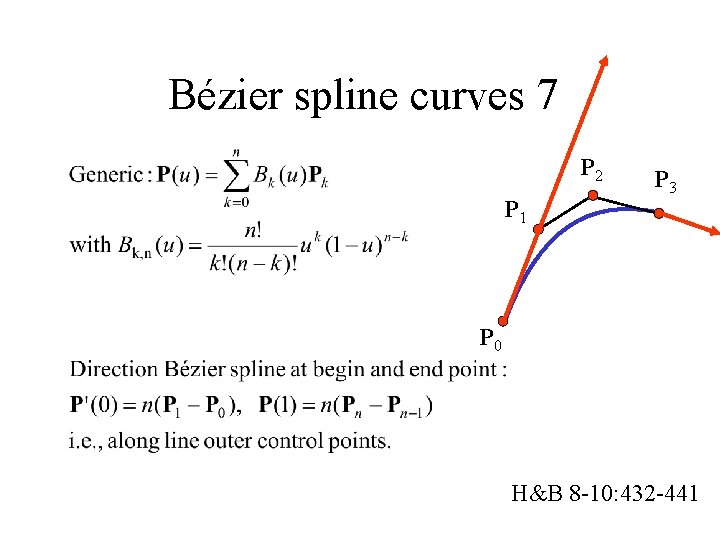
Bézier spline curves 7 P 2 P 1 P 3 P 0 H&B 8 -10: 432 -441

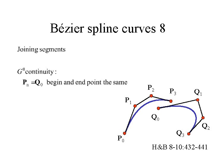
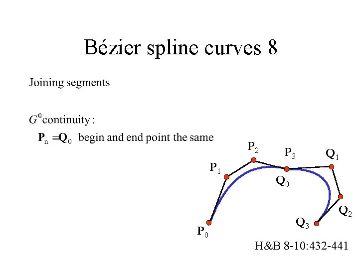
Bézier spline curves 8 P 2 P 1 P 3 Q 1 Q 0 P 0 Q 3 Q 2 H&B 8 -10: 432 -441

Bézier spline curves 8 P 2 P 1 P 0 P 3 Q 1 Q 0 Q 3 Q 2 H&B 8 -10: 432 -441

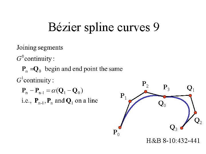
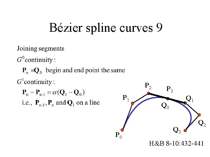
Bézier spline curves 9 P 2 P 1 P 0 P 3 Q 1 Q 0 Q 3 Q 2 H&B 8 -10: 432 -441

Bézier spline curves 9 P 2 P 1 P 0 P 3 Q 1 Q 0 Q 3 Q 2 H&B 8 -10: 432 -441

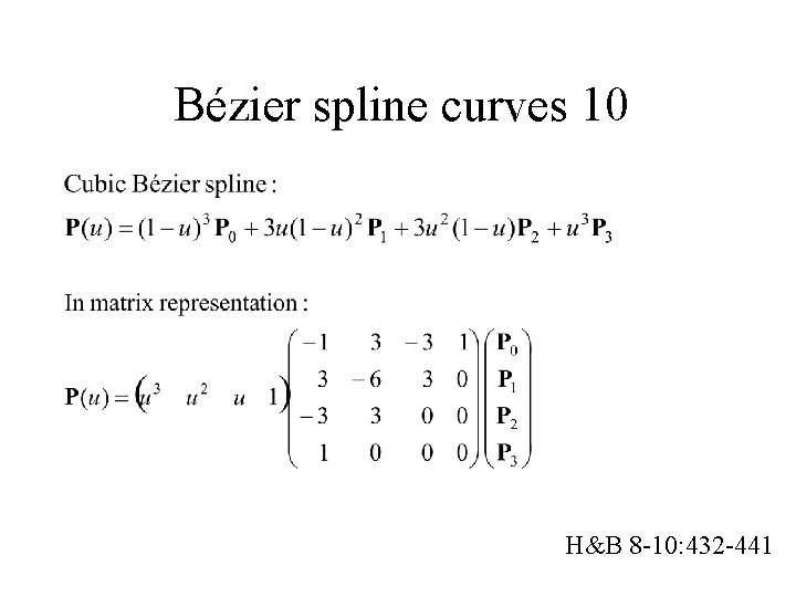
Bézier spline curves 10 H&B 8 -10: 432 -441

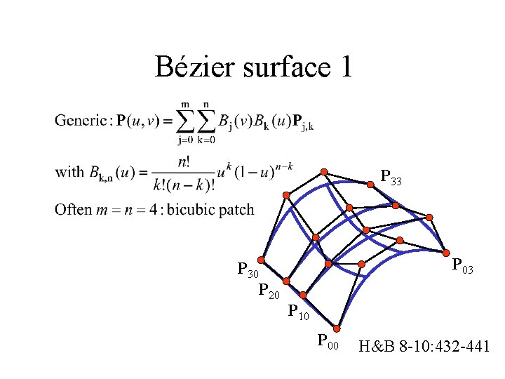
Bézier surface 1 P 33 P 30 P 20 P 03 P 10 P 00 H&B 8 -10: 432 -441

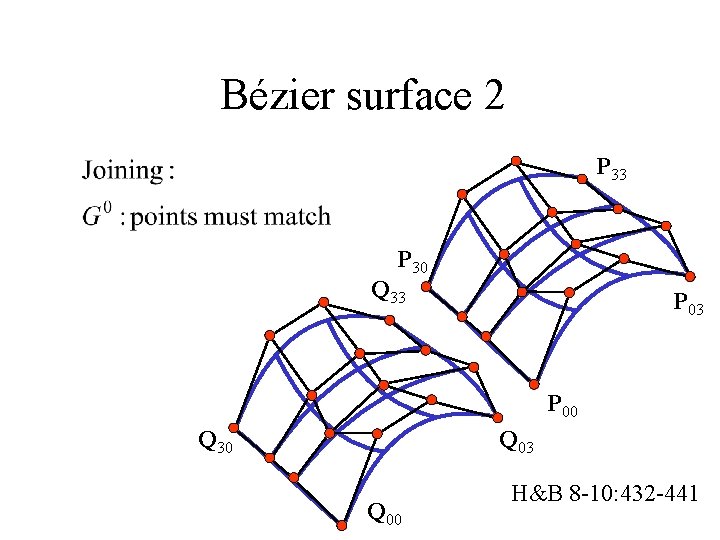
Bézier surface 2 P 33 P 30 Q 33 P 00 Q 03 Q 30 Q 00 H&B 8 -10: 432 -441

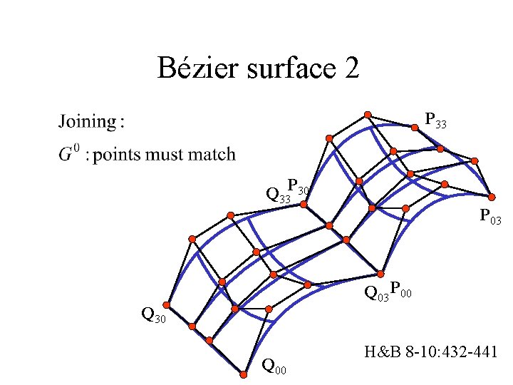
Bézier surface 2 P 33 Q 33 P 30 P 03 Q 03 P 00 Q 30 Q 00 H&B 8 -10: 432 -441

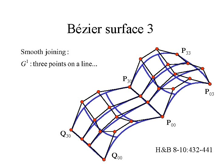
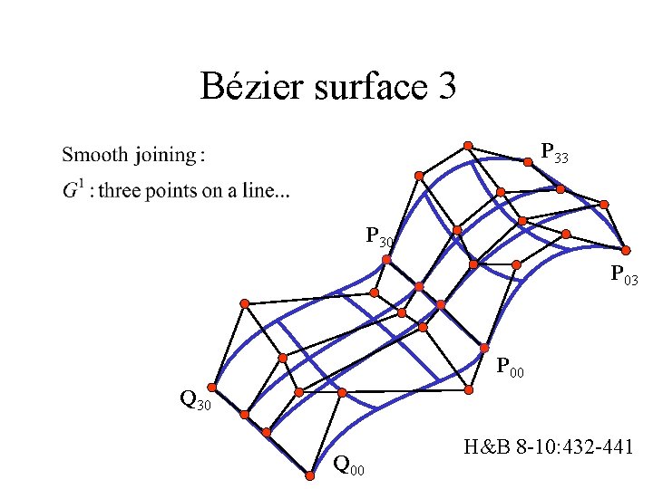
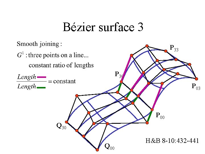
Bézier surface 3 P 30 P 03 P 00 Q 30 Q 00 H&B 8 -10: 432 -441

Bézier surface 3 P 30 P 03 P 00 Q 30 Q 00 H&B 8 -10: 432 -441

Bézier surface 3 P 30 P 03 P 00 Q 30 Q 00 H&B 8 -10: 432 -441

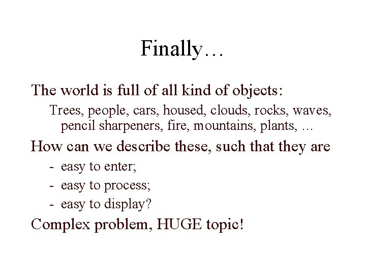
Finally… The world is full of all kind of objects: Trees, people, cars, housed, clouds, rocks, waves, pencil sharpeners, fire, mountains, plants, … How can we describe these, such that they are - easy to enter; - easy to process; - easy to display? Complex problem, HUGE topic!

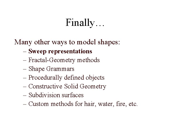
Finally… Many other ways to model shapes: – Sweep representations – Fractal-Geometry methods – Shape Grammars – Procedurally defined objects – Constructive Solid Geometry – Subdivision surfaces – Custom methods for hair, water, fire, etc.

Next… • We now know how to model curved objects • But they still look somewhat dull, …