2 IV 60 Computer graphics Graphics primitives and

2 IV 60 Computer graphics Graphics primitives and attributes Jack van Wijk TU/e

Overview • Basic graphics primitives: – points, lines, polygons • Basic attributes – linewidth, color

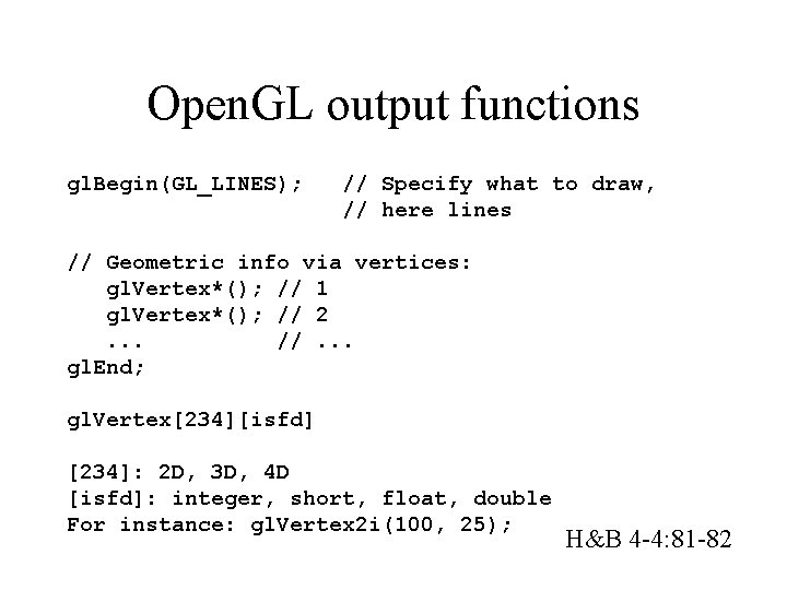
Open. GL output functions gl. Begin(GL_LINES); // Specify what to draw, // here lines // Geometric info via vertices: gl. Vertex*(); // 1 gl. Vertex*(); // 2. . . //. . . gl. End; gl. Vertex[234][isfd] [234]: 2 D, 3 D, 4 D [isfd]: integer, short, float, double For instance: gl. Vertex 2 i(100, 25); H&B 4 -4: 81 -82

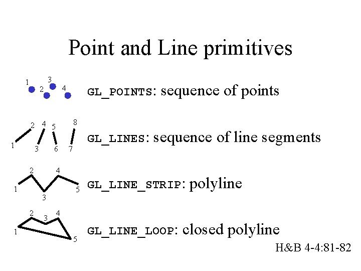
Point and Line primitives 3 1 GL_POINTS: 4 2 8 2 4 5 1 3 6 2 1 1 GL_LINES: 7 4 5 3 2 3 sequence of points sequence of line segments GL_LINE_STRIP: polyline 4 5 GL_LINE_LOOP: closed polyline H&B 4 -4: 81 -82

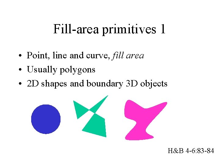
Fill-area primitives 1 • Point, line and curve, fill area • Usually polygons • 2 D shapes and boundary 3 D objects H&B 4 -6: 83 -84

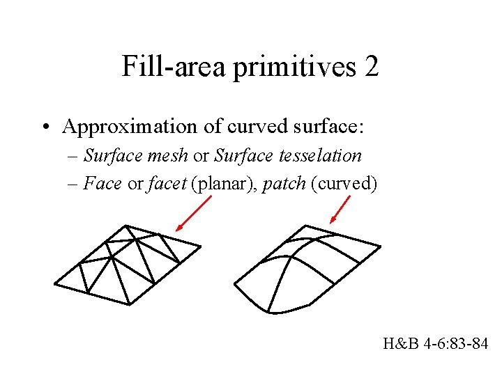
Fill-area primitives 2 • Approximation of curved surface: – Surface mesh or Surface tesselation – Face or facet (planar), patch (curved) H&B 4 -6: 83 -84

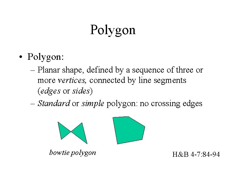
Polygon • Polygon: – Planar shape, defined by a sequence of three or more vertices, connected by line segments (edges or sides) – Standard or simple polygon: no crossing edges bowtie polygon H&B 4 -7: 84 -94

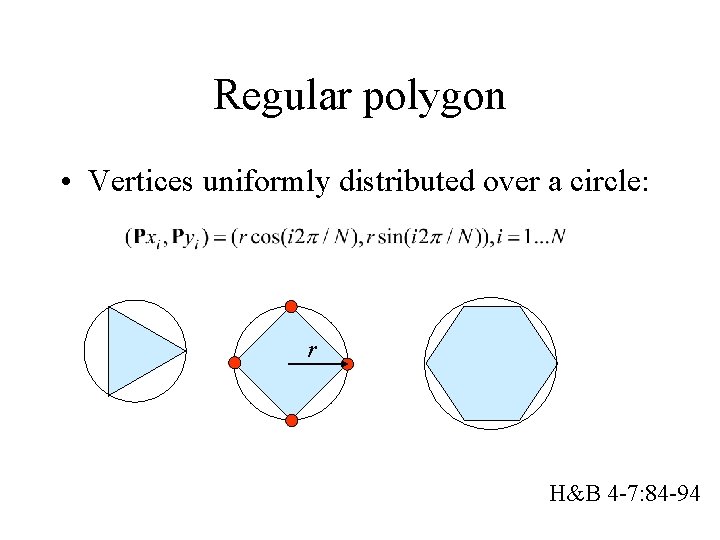
Regular polygon • Vertices uniformly distributed over a circle: r H&B 4 -7: 84 -94

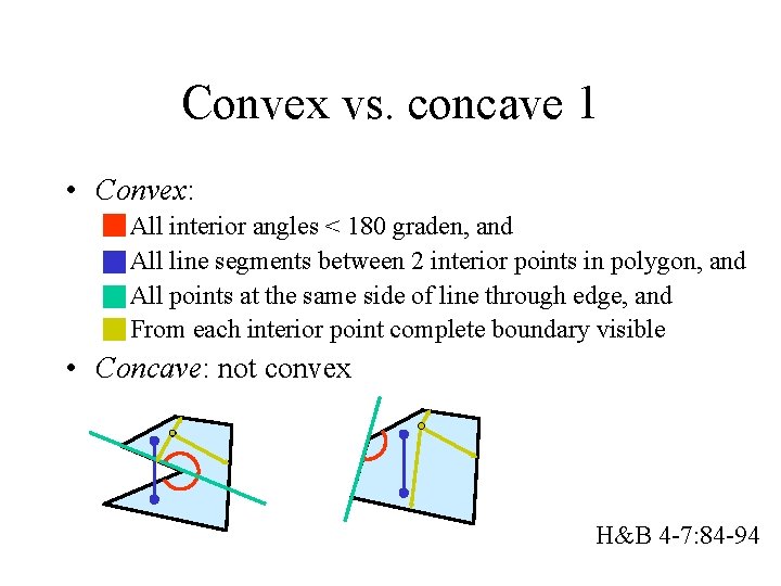
Convex vs. concave 1 • Convex: – – All interior angles < 180 graden, and All line segments between 2 interior points in polygon, and All points at the same side of line through edge, and From each interior point complete boundary visible • Concave: not convex H&B 4 -7: 84 -94

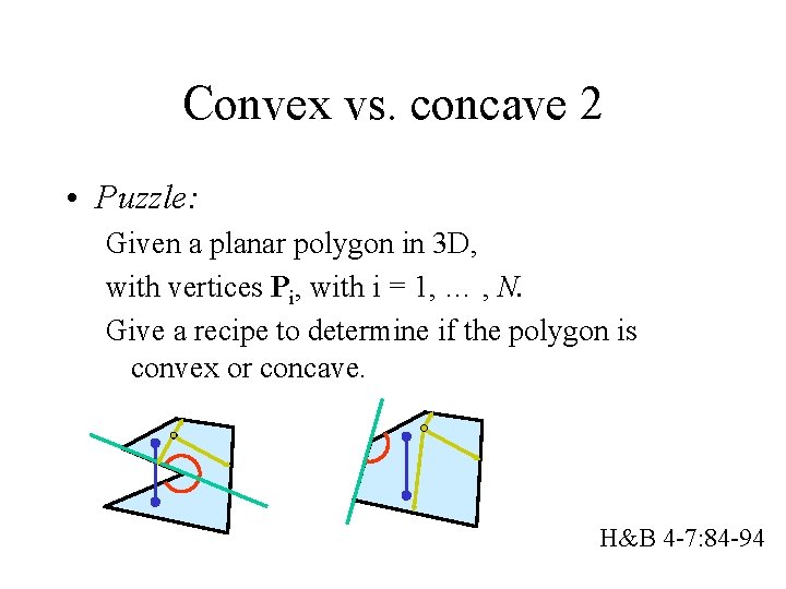
Convex vs. concave 2 • Puzzle: Given a planar polygon in 3 D, with vertices Pi, with i = 1, … , N. Give a recipe to determine if the polygon is convex or concave. H&B 4 -7: 84 -94

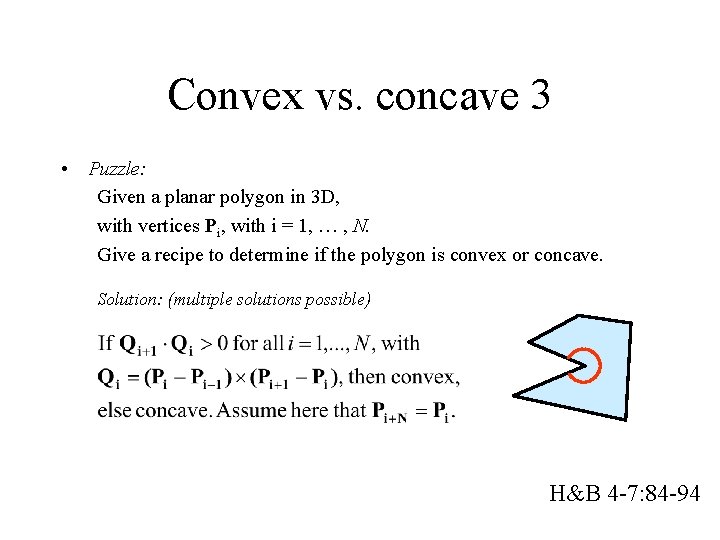
Convex vs. concave 3 • Puzzle: Given a planar polygon in 3 D, with vertices Pi, with i = 1, … , N. Give a recipe to determine if the polygon is convex or concave. Solution: (multiple solutions possible) H&B 4 -7: 84 -94

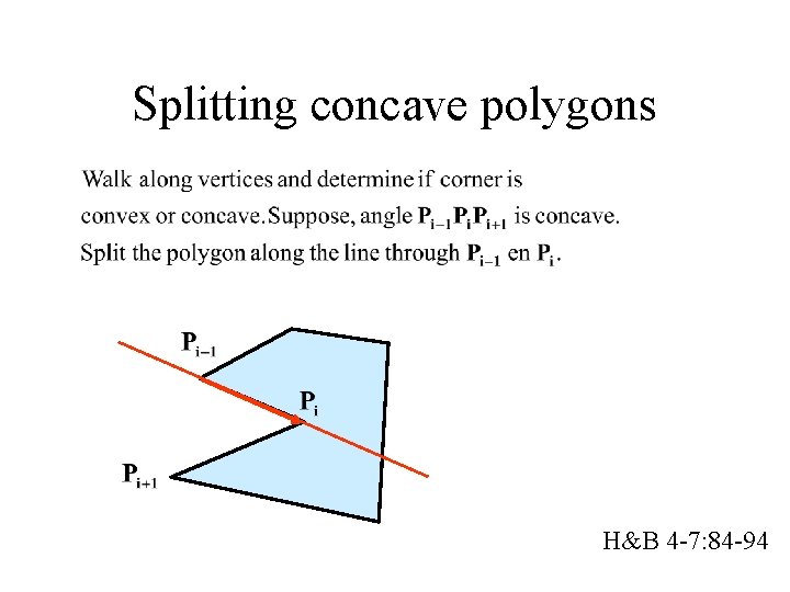
Splitting concave polygons H&B 4 -7: 84 -94

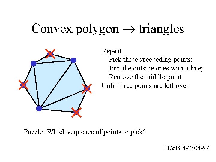
Convex polygon triangles Repeat Pick three succeeding points; Join the outside ones with a line; Remove the middle point Until three points are left over Puzzle: Which sequence of points to pick? H&B 4 -7: 84 -94

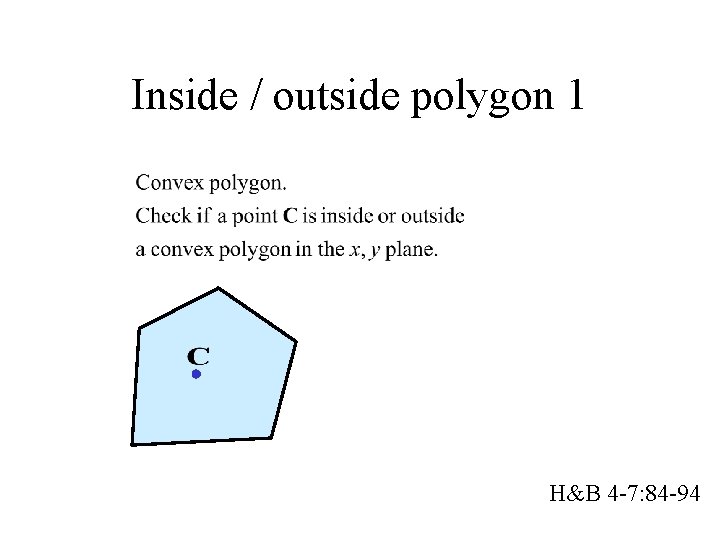
Inside / outside polygon 1 H&B 4 -7: 84 -94

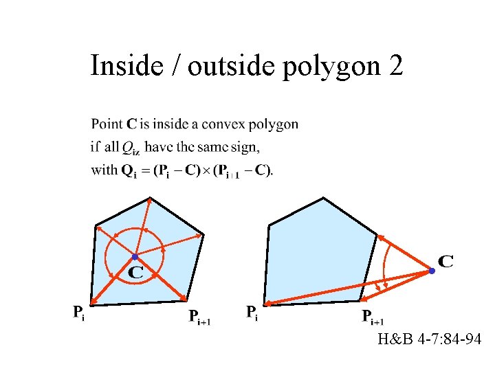
Inside / outside polygon 2 H&B 4 -7: 84 -94

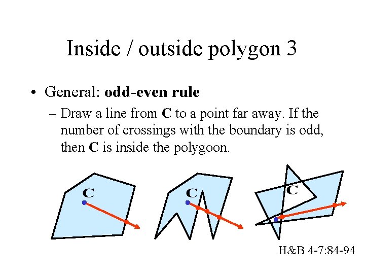
Inside / outside polygon 3 • General: odd-even rule – Draw a line from C to a point far away. If the number of crossings with the boundary is odd, then C is inside the polygoon. H&B 4 -7: 84 -94

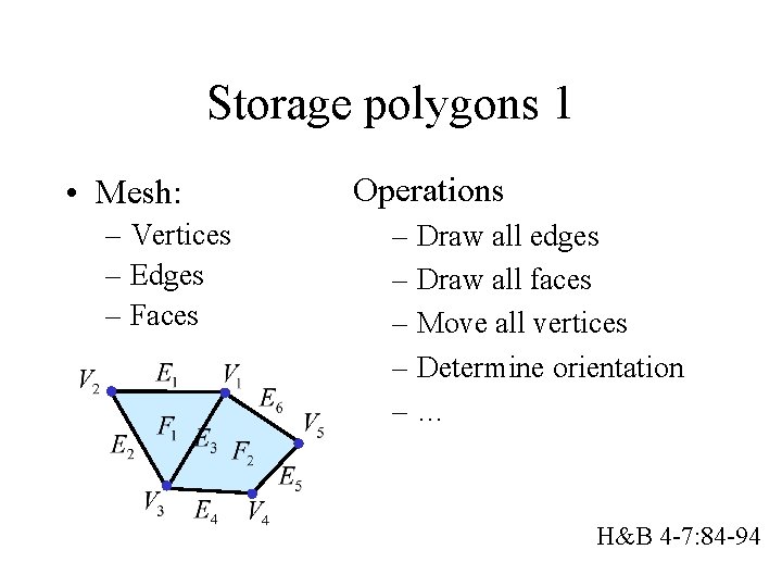
Storage polygons 1 • Mesh: – Vertices – Edges – Faces Operations – Draw all edges – Draw all faces – Move all vertices – Determine orientation –… H&B 4 -7: 84 -94

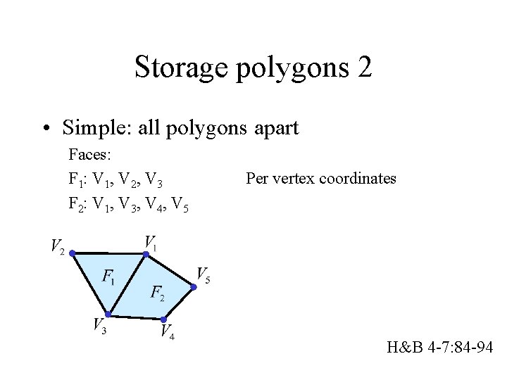
Storage polygons 2 • Simple: all polygons apart Faces: F 1: V 1, V 2, V 3 F 2: V 1, V 3, V 4, V 5 Per vertex coordinates H&B 4 -7: 84 -94

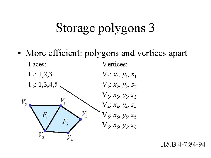
Storage polygons 3 • More efficient: polygons and vertices apart Faces: F 1: 1, 2, 3 F 2: 1, 3, 4, 5 Vertices: V 1: x 1, y 1, z 1 V 2: x 2, y 2, z 2 V 3: x 3, y 3, z 3 V 4: x 4, y 4, z 4 V 5: x 5, y 5, z 5 V 6: x 6, y 6, z 6 H&B 4 -7: 84 -94

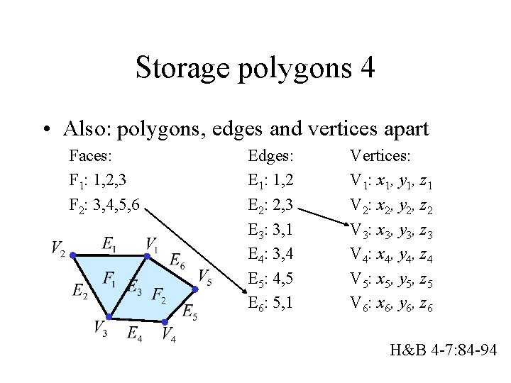
Storage polygons 4 • Also: polygons, edges and vertices apart Faces: F 1: 1, 2, 3 F 2: 3, 4, 5, 6 Edges: E 1: 1, 2 E 2: 2, 3 E 3: 3, 1 E 4: 3, 4 E 5: 4, 5 E 6: 5, 1 Vertices: V 1: x 1, y 1, z 1 V 2: x 2, y 2, z 2 V 3: x 3, y 3, z 3 V 4: x 4, y 4, z 4 V 5: x 5, y 5, z 5 V 6: x 6, y 6, z 6 H&B 4 -7: 84 -94

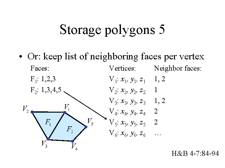
Storage polygons 5 • Or: keep list of neighboring faces per vertex Faces: F 1: 1, 2, 3 F 2: 1, 3, 4, 5 Vertices: V 1: x 1, y 1, z 1 V 2: x 2, y 2, z 2 V 3: x 3, y 3, z 3 V 4: x 4, y 4, z 4 V 5: x 5, y 5, z 5 V 6: x 6, y 6, z 6 Neighbor faces: 1, 2 1 1, 2 2 2 … H&B 4 -7: 84 -94

Storage polygons 6 • Many other formats possible – See f. i. winged edge data structure • Select/design storage format based on: – Operations on elements; – Efficiency (size and operations); – Simplicity – Maintainability – Consistency –… H&B 4 -7: 84 -94

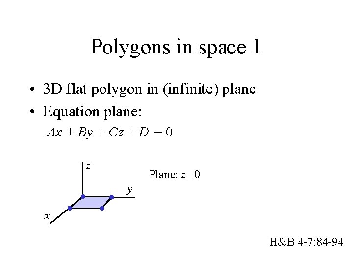
Polygons in space 1 • 3 D flat polygon in (infinite) plane • Equation plane: Ax + By + Cz + D = 0 z Plane: z=0 y x H&B 4 -7: 84 -94

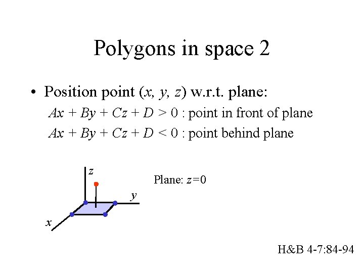
Polygons in space 2 • Position point (x, y, z) w. r. t. plane: Ax + By + Cz + D > 0 : point in front of plane Ax + By + Cz + D < 0 : point behind plane z Plane: z=0 y x H&B 4 -7: 84 -94

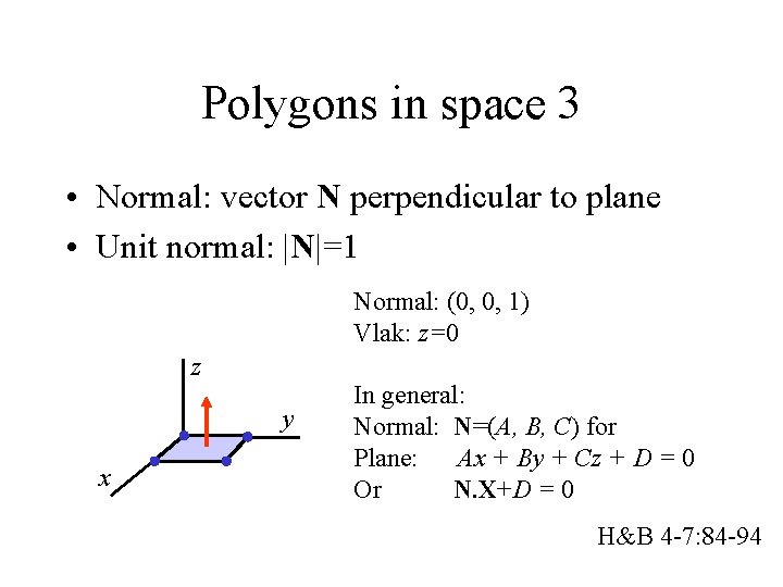
Polygons in space 3 • Normal: vector N perpendicular to plane • Unit normal: |N|=1 Normal: (0, 0, 1) Vlak: z=0 z y x In general: Normal: N=(A, B, C) for Plane: Ax + By + Cz + D = 0 Or N. X+D = 0 H&B 4 -7: 84 -94

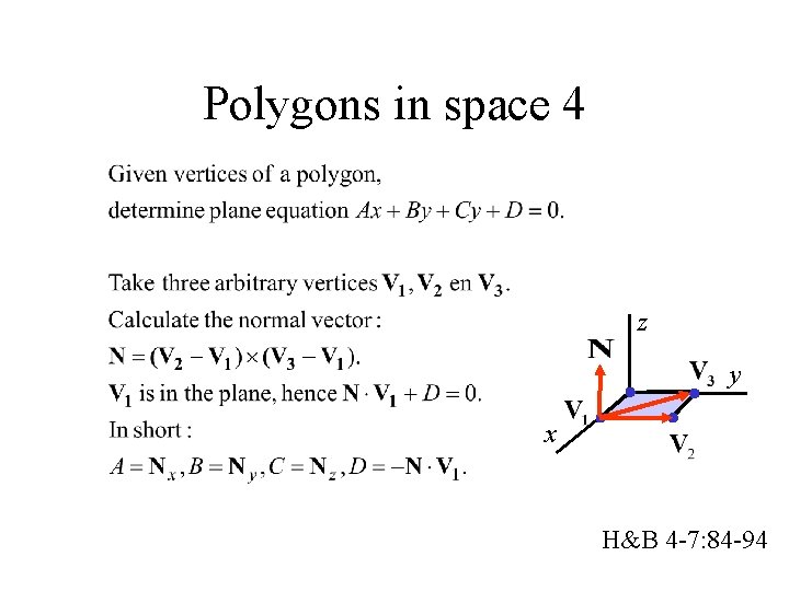
Polygons in space 4 z y x H&B 4 -7: 84 -94

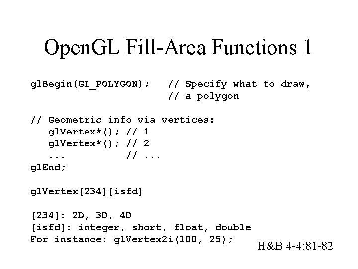
Open. GL Fill-Area Functions 1 gl. Begin(GL_POLYGON); // Specify what to draw, // a polygon // Geometric info via vertices: gl. Vertex*(); // 1 gl. Vertex*(); // 2. . . //. . . gl. End; gl. Vertex[234][isfd] [234]: 2 D, 3 D, 4 D [isfd]: integer, short, float, double For instance: gl. Vertex 2 i(100, 25); H&B 4 -4: 81 -82

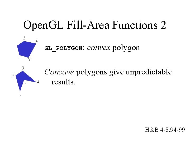
Open. GL Fill-Area Functions 2 3 1 4 GL_POLYGON: convex polygon 5 3 2 5 4 Concave polygons give unpredictable results. 1 H&B 4 -8: 94 -99

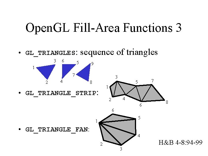
Open. GL Fill-Area Functions 3 • GL_TRIANGLES: 3 6 sequence of triangles 5 1 9 7 2 4 3 8 1 • GL_TRIANGLE_STRIP: 7 5 4 2 6 8 6 5 1 • GL_TRIANGLE_FAN: 4 2 H&B 4 -8: 94 -99 3

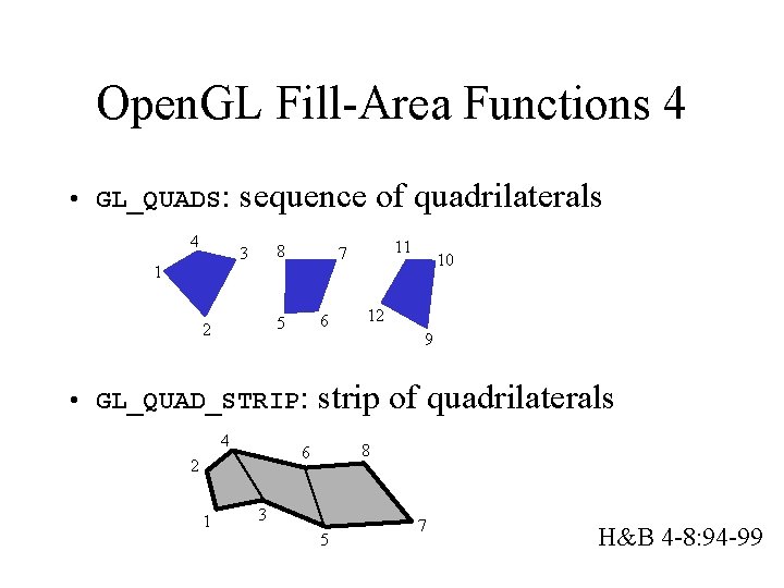
Open. GL Fill-Area Functions 4 • GL_QUADS: 4 sequence of quadrilaterals 8 3 1 6 5 2 • GL_QUAD_STRIP: 4 1 10 12 9 strip of quadrilaterals 8 6 2 11 7 3 5 7 H&B 4 -8: 94 -99

More efficiency • Reduce the number of function calls: – Open. GL Vertex Arrays: pass arrays of vertices instead of single ones; • Store information on GPU and do not resend: – Open. GL Display lists; – Vertex Buffer Objects. H&B App. C

Open. GL Display lists 1 Key idea: Collect a sequence of Open. GL commands in a structure, stored at the GPU, and reference it later on + Simple to program + Can give a boost + Useful for static scenes and hierarchical models Not the most modern H&B 4 -15 111 -113

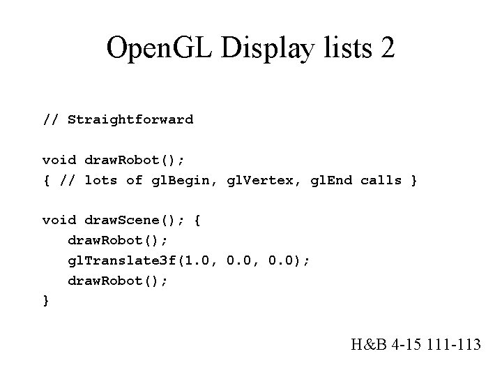
Open. GL Display lists 2 // Straightforward void draw. Robot(); { // lots of gl. Begin, gl. Vertex, gl. End calls } void draw. Scene(); { draw. Robot(); gl. Translate 3 f(1. 0, 0. 0); draw. Robot(); } H&B 4 -15 111 -113

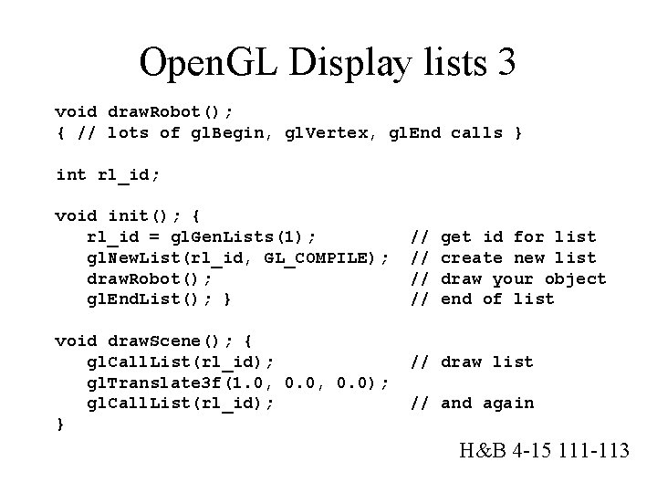
Open. GL Display lists 3 void draw. Robot(); { // lots of gl. Begin, gl. Vertex, gl. End calls } int rl_id; void init(); { rl_id = gl. Gen. Lists(1); gl. New. List(rl_id, GL_COMPILE); draw. Robot(); gl. End. List(); } void draw. Scene(); { gl. Call. List(rl_id); gl. Translate 3 f(1. 0, 0. 0); gl. Call. List(rl_id); } // // get id for list create new list draw your object end of list // draw list // and again H&B 4 -15 111 -113

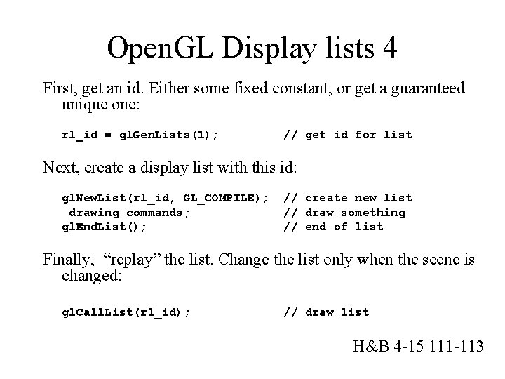
Open. GL Display lists 4 First, get an id. Either some fixed constant, or get a guaranteed unique one: rl_id = gl. Gen. Lists(1); // get id for list Next, create a display list with this id: gl. New. List(rl_id, GL_COMPILE); drawing commands; gl. End. List(); // create new list // draw something // end of list Finally, “replay” the list. Change the list only when the scene is changed: gl. Call. List(rl_id); // draw list H&B 4 -15 111 -113

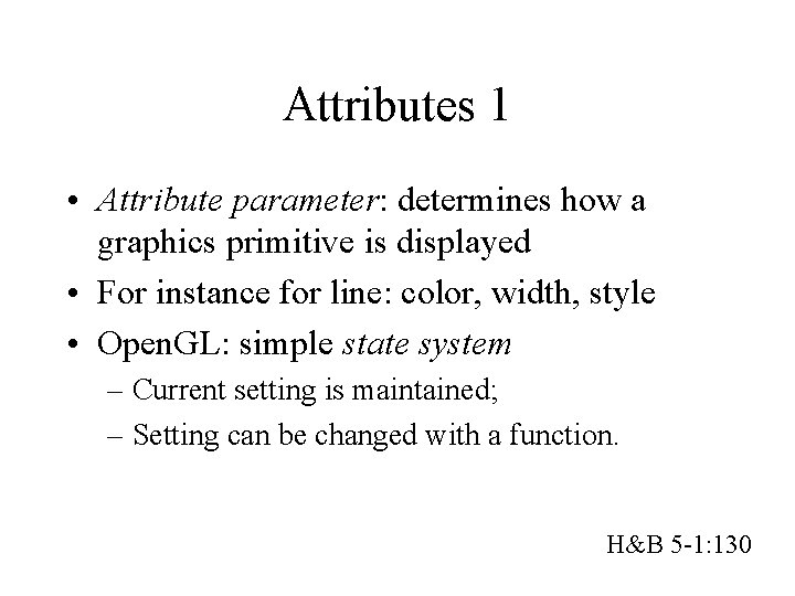
Attributes 1 • Attribute parameter: determines how a graphics primitive is displayed • For instance for line: color, width, style • Open. GL: simple state system – Current setting is maintained; – Setting can be changed with a function. H&B 5 -1: 130

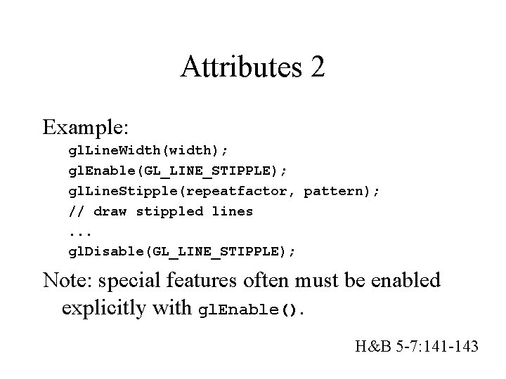
Attributes 2 Example: gl. Line. Width(width); gl. Enable(GL_LINE_STIPPLE); gl. Line. Stipple(repeatfactor, pattern); // draw stippled lines. . . gl. Disable(GL_LINE_STIPPLE); Note: special features often must be enabled explicitly with gl. Enable(). H&B 5 -7: 141 -143

Color 1 RGB mode : • color = (red, green, blue) • gl. Color[34][bisf]: set color of vertex • For example: – gl. Color 4 f(red, green, blue, alpha) – alpha: opacity (1 transparantie) H&B 5 -2: 130 -131

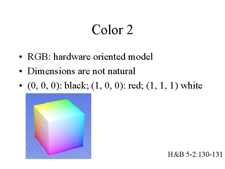
Color 2 • RGB: hardware oriented model • Dimensions are not natural • (0, 0, 0): black; (1, 0, 0): red; (1, 1, 1) white H&B 5 -2: 130 -131

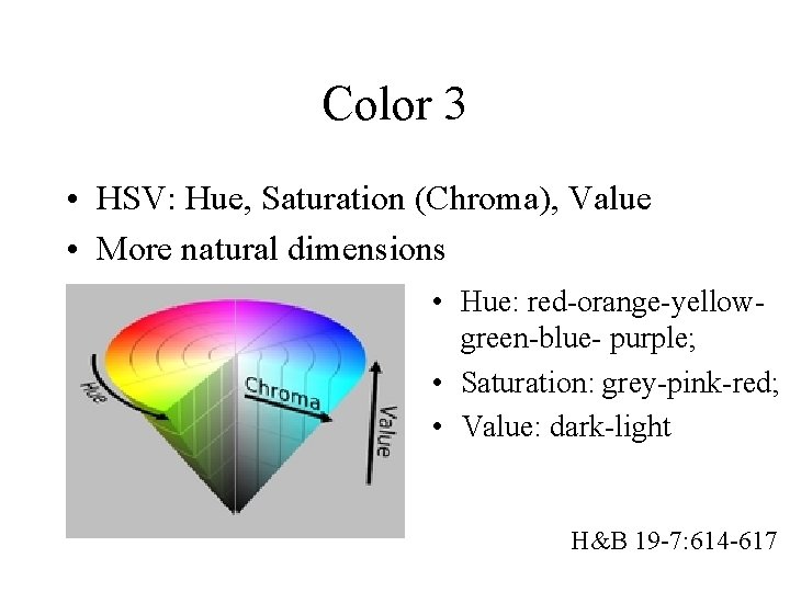
Color 3 • HSV: Hue, Saturation (Chroma), Value • More natural dimensions • Hue: red-orange-yellowgreen-blue- purple; • Saturation: grey-pink-red; • Value: dark-light H&B 19 -7: 614 -617

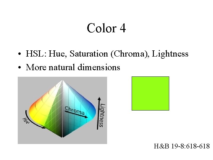
Color 4 • HSL: Hue, Saturation (Chroma), Lightness • More natural dimensions H&B 19 -8: 618 -618

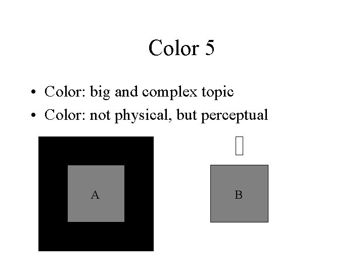
Color 5 • Color: big and complex topic • Color: not physical, but perceptual A B

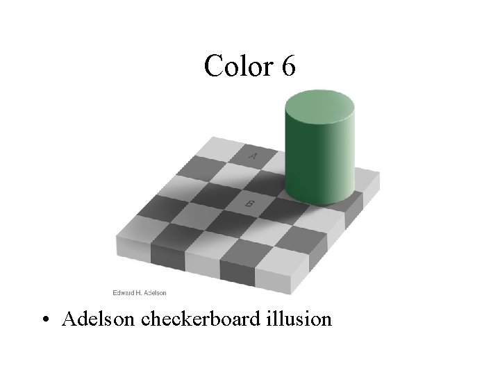
Color 6 • Adelson checkerboard illusion

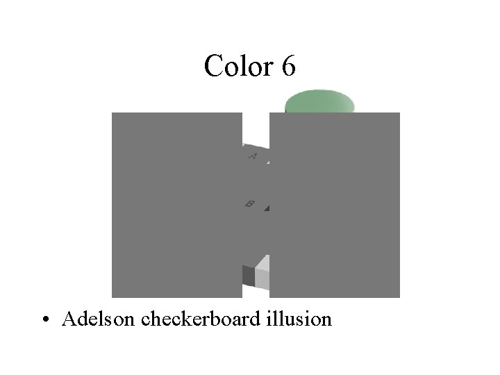
Color 6 • Adelson checkerboard illusion

Next • We now know how to draw polygons. • How to model geometric objects?