2 Introduction to Rosetta and structural modeling The

2. Introduction to Rosetta and structural modeling • The Rosetta framework • Scoring (selecting the structure) and • Sampling (finding the structure) • Cartesian and polar coordinates

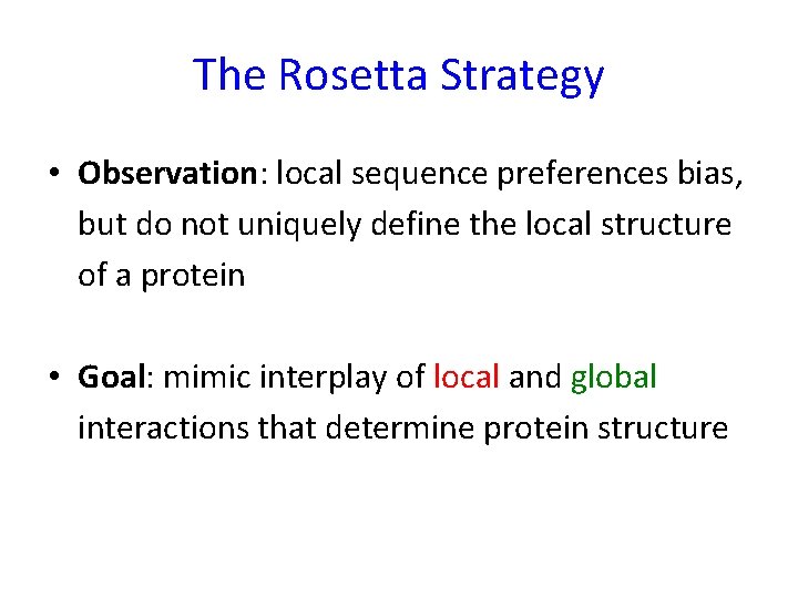
The Rosetta Strategy • Observation: local sequence preferences bias, but do not uniquely define the local structure of a protein • Goal: mimic interplay of local and global interactions that determine protein structure

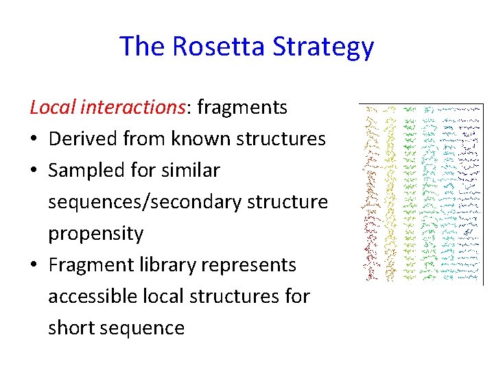
The Rosetta Strategy Local interactions: fragments • Derived from known structures • Sampled for similar sequences/secondary structure propensity • Fragment library represents accessible local structures for short sequence

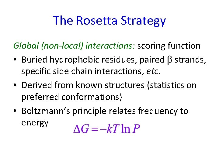
The Rosetta Strategy Global (non-local) interactions: scoring function • Buried hydrophobic residues, paired strands, specific side chain interactions, etc. • Derived from known structures (statistics on preferred conformations) • Boltzmann’s principle relates frequency to energy

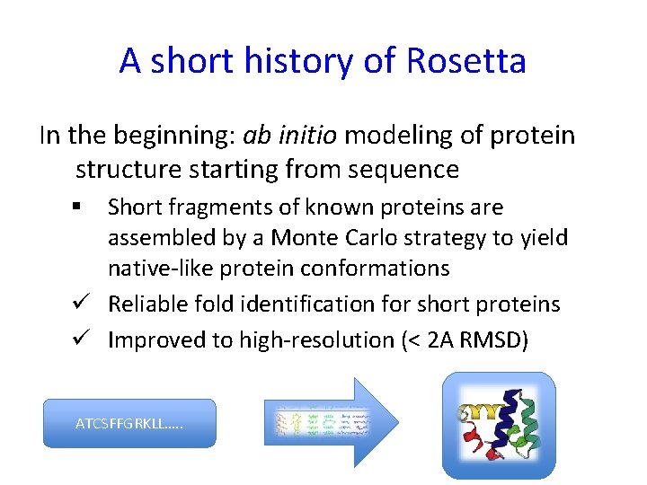
A short history of Rosetta In the beginning: ab initio modeling of protein structure starting from sequence § Short fragments of known proteins are assembled by a Monte Carlo strategy to yield native-like protein conformations ü Reliable fold identification for short proteins ü Improved to high-resolution (< 2 A RMSD) ATCSFFGRKLL…. .

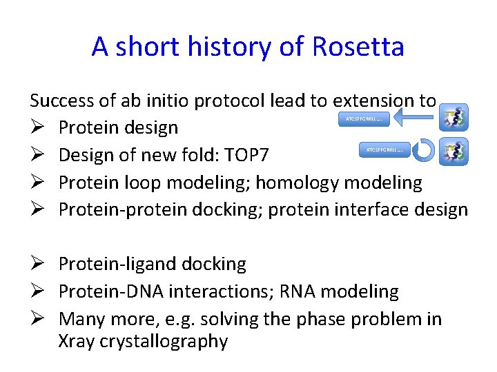
A short history of Rosetta Success of ab initio protocol lead to extension to Ø Protein design Ø Design of new fold: TOP 7 Ø Protein loop modeling; homology modeling Ø Protein-protein docking; protein interface design ATCSFFGRKLL…. . Ø Protein-ligand docking Ø Protein-DNA interactions; RNA modeling Ø Many more, e. g. solving the phase problem in Xray crystallography

Rosetta extensions • Boinc (Rosetta@home) • Fold. It • Rosettascripts • Py. Rosetta

Scoring and Sampling

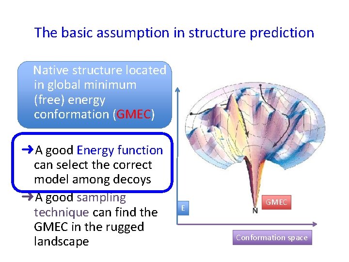
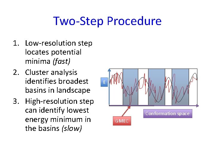
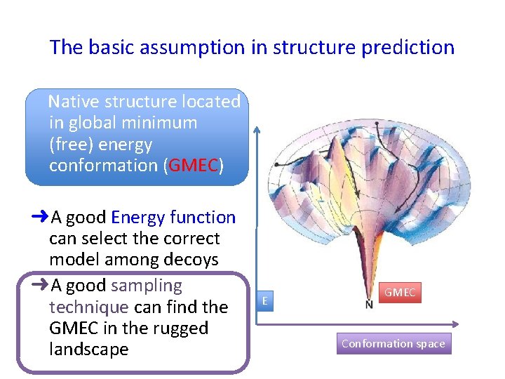
The basic assumption in structure prediction Native structure located in global minimum (free) energy conformation (GMEC) ➜A good Energy function can select the correct model among decoys ➜A good sampling technique can find the GMEC in the rugged landscape E GMEC Conformation space

Two-Step Procedure 1. Low-resolution step locates potential minima (fast) 2. Cluster analysis identifies broadest basins in landscape 3. High-resolution step can identify lowest energy minimum in the basins (slow) E Conformation space GMEC

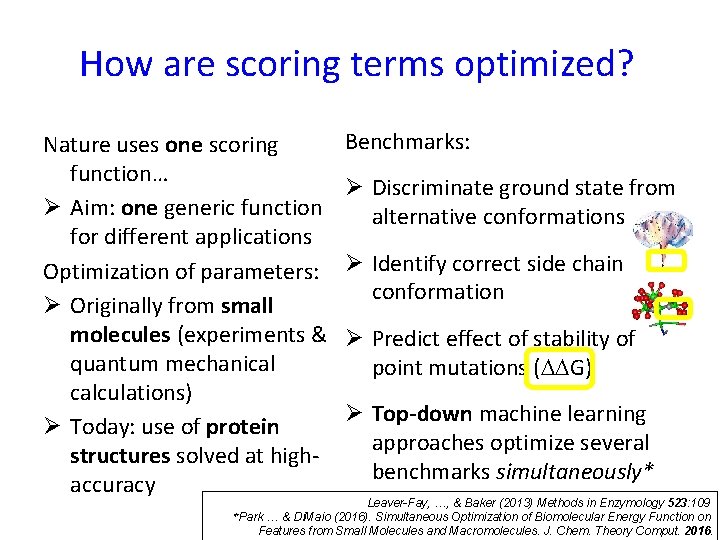
How are scoring terms optimized? Nature uses one scoring function… Ø Aim: one generic function for different applications Optimization of parameters: Ø Originally from small molecules (experiments & quantum mechanical calculations) Ø Today: use of protein structures solved at highaccuracy Benchmarks: Ø Discriminate ground state from alternative conformations Ø Identify correct side chain conformation Ø Predict effect of stability of point mutations (DDG) Ø Top-down machine learning approaches optimize several benchmarks simultaneously* Leaver-Fay, …, & Baker (2013) Methods in Enzymology 523: 109 *Park … & Di. Maio (2016). Simultaneous Optimization of Biomolecular Energy Function on Features from Small Molecules and Macromolecules. J. Chem. Theory Comput. 2016.

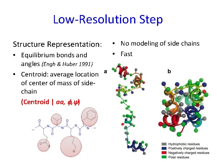
Low-Resolution Step Structure Representation: • Equilibrium bonds and angles (Engh & Huber 1991) • Centroid: average location of center of mass of sidechain (Centroid | aa, f, ) • No modeling of side chains • Fast

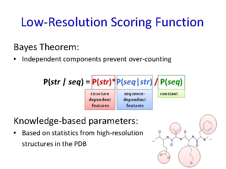
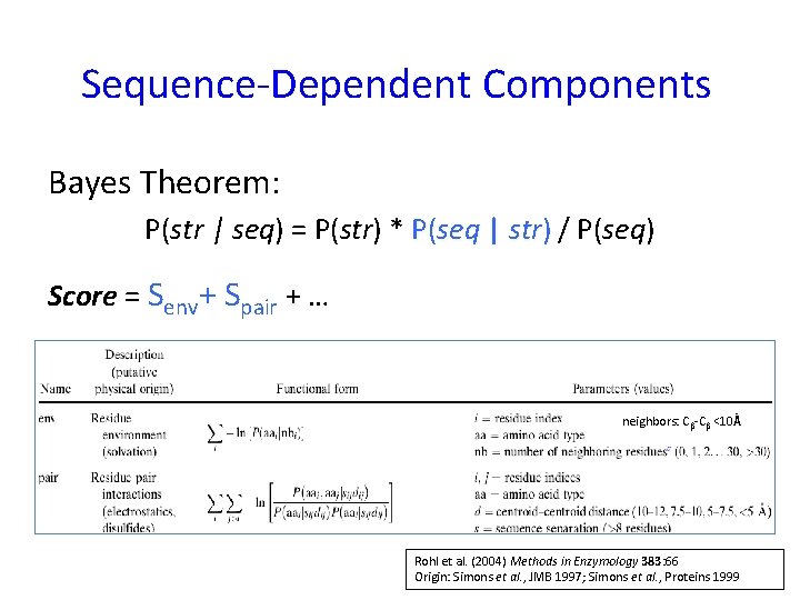
Low-Resolution Scoring Function Bayes Theorem: • Independent components prevent over-counting P(str | seq) = P(str)*P(seq|str) / P(seq) structure dependent features sequencedependent features Knowledge-based parameters: • Based on statistics from high-resolution structures in the PDB constant

Sequence-Dependent Components Bayes Theorem: P(str | seq) = P(str) * P(seq | str) / P(seq) Score = Senv+ Spair + … neighbors: C -C <10Ǻ Rohl et al. (2004) Methods in Enzymology 383: 66 Origin: Simons et al. , JMB 1997; Simons et al. , Proteins 1999

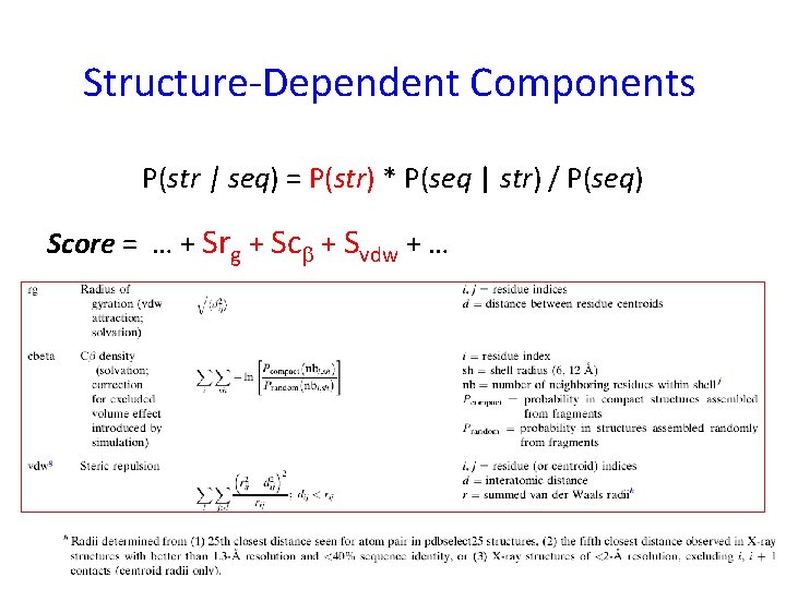
Structure-Dependent Components P(str | seq) = P(str) * P(seq | str) / P(seq) Score = … + Srg + Sc + Svdw + …

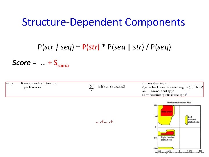
Structure-Dependent Components P(str | seq) = P(str) * P(seq | str) / P(seq) Score = … + Srama 10 …. +…. . +

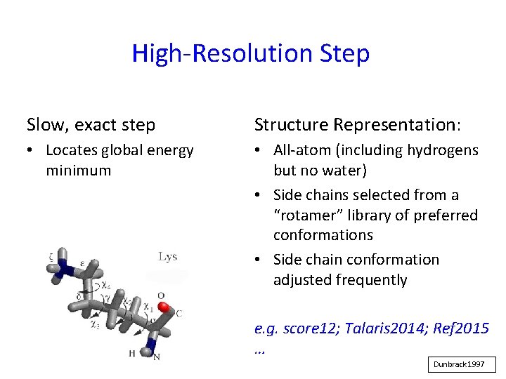
High-Resolution Step Slow, exact step Structure Representation: • Locates global energy minimum • All-atom (including hydrogens but no water) • Side chains selected from a “rotamer” library of preferred conformations • Side chain conformation adjusted frequently e. g. score 12; Talaris 2014; Ref 2015 … Dunbrack 1997

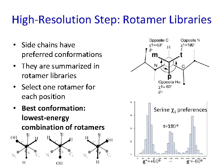
High-Resolution Step: Rotamer Libraries • Side chains have preferred conformations • They are summarized in rotamer libraries • Select one rotamer for each position • Best conformation: lowest-energy combination of rotamers Serine c 1 preferences t=180 o g+=+60 o g-=-60 o

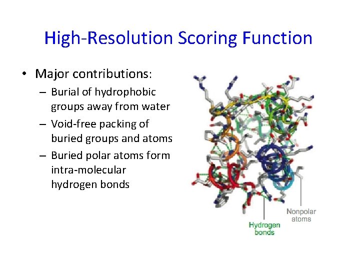
High-Resolution Scoring Function • Major contributions: – Burial of hydrophobic groups away from water – Void-free packing of buried groups and atoms – Buried polar atoms form intra-molecular hydrogen bonds

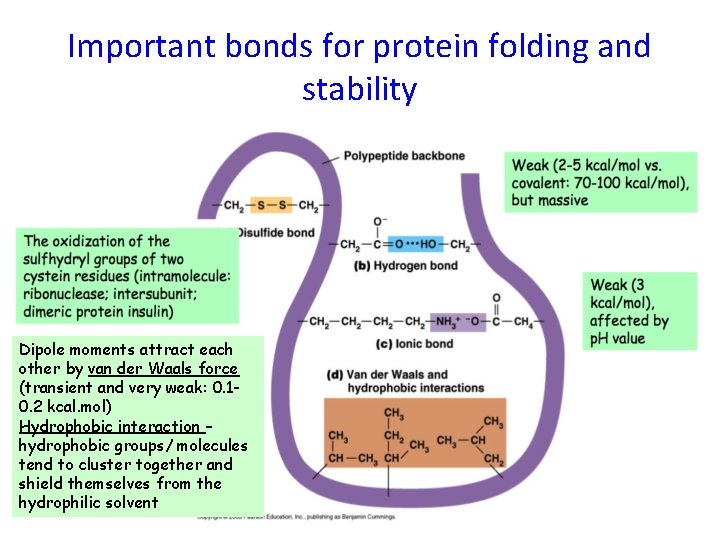
Important bonds for protein folding and stability Dipole moments attract each other by van der Waals force (transient and very weak: 0. 10. 2 kcal. mol) Hydrophobic interaction – hydrophobic groups/ molecules tend to cluster together and shield themselves from the hydrophilic solvent

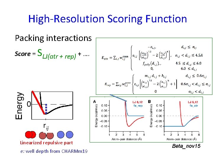
High-Resolution Scoring Function Packing interactions Score = SLJ(atr + rep) + …. rij Linearized repulsive part e: well depth from CHARMm 19 Beta_nov 15

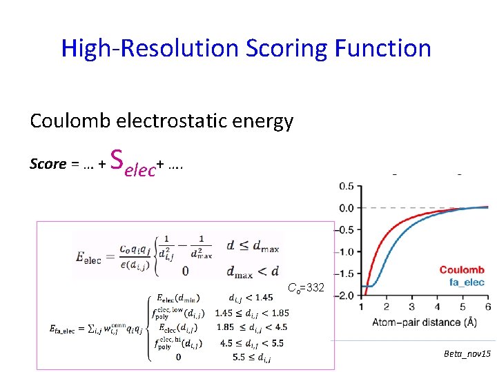
High-Resolution Scoring Function Coulomb electrostatic energy Score = … + Selec+ …. Co=332 Beta_nov 15

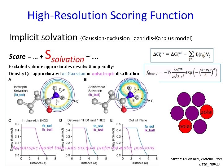
High-Resolution Scoring Function Implicit solvation (Gaussian-exclusion Lazaridis-Karplus model) Score = … + Ssolvation + …. Excluded volume approximates desolvation penalty; Density f(r) approximated as Gaussian or anisotropic distribution polar Anisotropic model takes into account preferred water positions Lazaridis & Karplus, Proteins 1999 Beta_nov 15

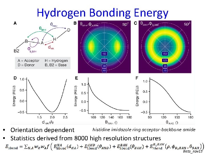
Hydrogen Bonding Energy histidine imidazole ring acceptor-backbone amide • Orientation dependent • Statistics derived from 8000 high resolution structures Beta_nov 15

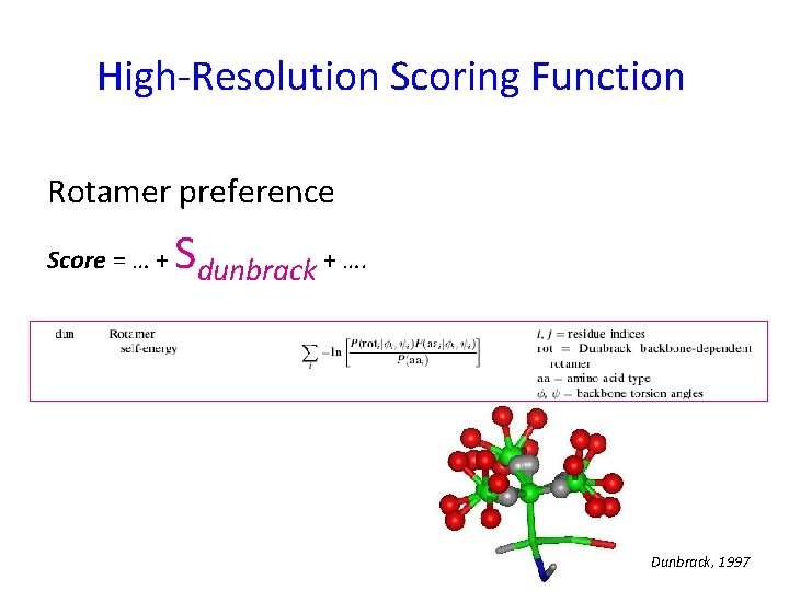
High-Resolution Scoring Function Rotamer preference Score = … + Sdunbrack + …. Dunbrack, 1997

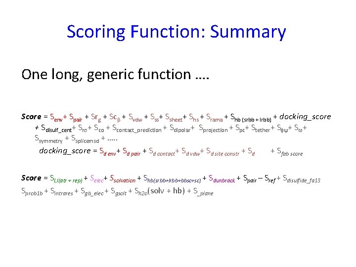
Scoring Function: Summary One long, generic function …. Score = Senv+ Spair + Srg + Sc + Svdw + Sss+ Ssheet+ Shs + Srama + Shb (srbb + lrbb) + docking_score + Sdisulf_cent+ Srs+ Scontact_prediction + Sdipolar+ Sprojection + Spc+ Stether+ Sfy+ Sw+ Ssymmetry + Ssplicemsd + …. . docking_score = Sd env+ Sd pair + Sd contact+ Sd vdw+ Sd site constr + Sd + Sfab score Score = SLJ(atr + rep) + Selec+ Ssolvation + Shb(srbb+lrbb+bbsc+sc) + Sdunbrack + Spair – Sref + Sdisulfide_fa 13 Sprob 1 b + Sintrares + Sgb_elec + Sgsolt + Sh 2 o(solv + hb) + S_plane

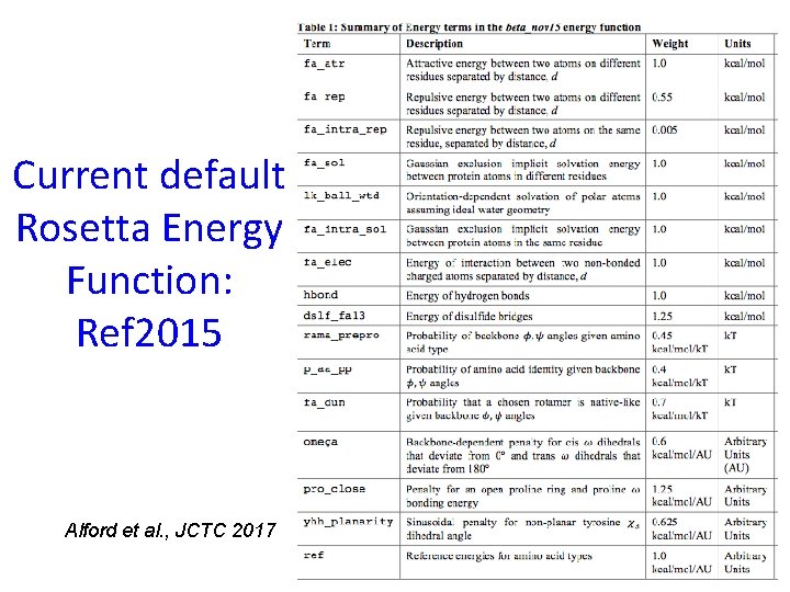
Current default Rosetta Energy Function: Ref 2015 Alford et al. , JCTC 2017

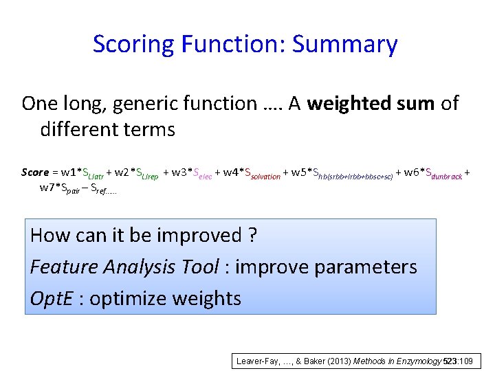
Scoring Function: Summary One long, generic function …. A weighted sum of different terms Score = w 1*SLJatr + w 2*SLJrep + w 3*Selec + w 4*Ssolvation + w 5*Shb(srbb+lrbb+bbsc+sc) + w 6*Sdunbrack + w 7*Spair – Sref…… How can it be improved ? Feature Analysis Tool : improve parameters Opt. E : optimize weights Leaver-Fay, …, & Baker (2013) Methods in Enzymology 523: 109

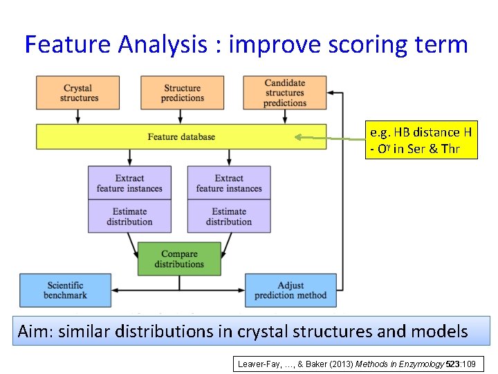
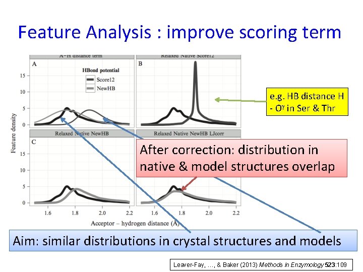
Feature Analysis : improve scoring term e. g. HB distance H - Og in Ser & Thr Aim: similar distributions in crystal structures and models Leaver-Fay, …, & Baker (2013) Methods in Enzymology 523: 109

Feature Analysis : improve scoring term e. g. HB distance H - Og in Ser & Thr After correction: distribution in native & model structures overlap Aim: similar distributions in crystal structures and models Leaver-Fay, …, & Baker (2013) Methods in Enzymology 523: 109

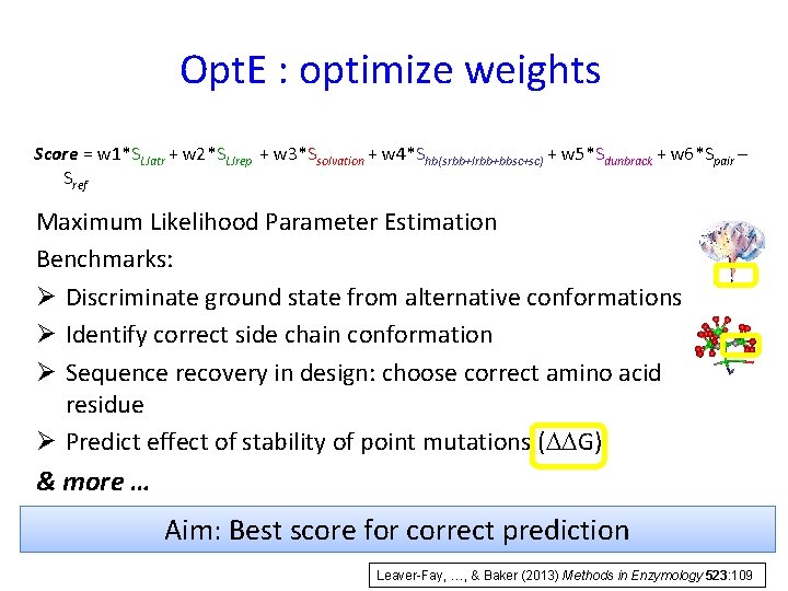
Opt. E : optimize weights Score = w 1*SLJatr + w 2*SLJrep + w 3*Ssolvation + w 4*Shb(srbb+lrbb+bbsc+sc) + w 5*Sdunbrack + w 6*Spair – Sref Maximum Likelihood Parameter Estimation Benchmarks: Ø Discriminate ground state from alternative conformations Ø Identify correct side chain conformation Ø Sequence recovery in design: choose correct amino acid residue Ø Predict effect of stability of point mutations (DDG) & more … Aim: Best score for correct prediction Leaver-Fay, …, & Baker (2013) Methods in Enzymology 523: 109

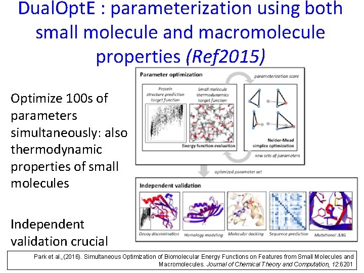
Dual. Opt. E : parameterization using both small molecule and macromolecule properties (Ref 2015) Optimize 100 s of parameters simultaneously: also thermodynamic properties of small molecules Independent validation crucial Park et al. , (2016). Simultaneous Optimization of Biomolecular Energy Functions on Features from Small Molecules and Macromolecules. Journal of Chemical Theory and Computation, 12: 6201

Scoring and Sampling

The basic assumption in structure prediction Native structure located in global minimum (free) energy conformation (GMEC) ➜A good Energy function can select the correct model among decoys ➜A good sampling technique can find the GMEC in the rugged landscape E GMEC Conformation space

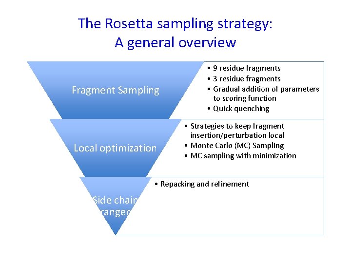
The Rosetta sampling strategy: A general overview Fragment Sampling Local optimization • 9 residue fragments • 3 residue fragments • Gradual addition of parameters to scoring function • Quick quenching • Strategies to keep fragment insertion/perturbation local • Monte Carlo (MC) Sampling • MC sampling with minimization • Repacking and refinement Side chain rearrangement

Representations of protein structure. Cartesian and polar coordinates PDB x ATOM …. 490 491 492 493 y N GLN A 31 CA GLN A 31 C GLN A 31 O GLN A 31 z 52. 013 -87. 359 -8. 797 1. 00 7. 06 52. 134 -87. 762 -10. 201 1. 00 8. 67 51. 726 -89. 222 -10. 343 1. 00 10. 90 51. 015 -89. 601 -11. 275 1. 00 9. 63 N C C O Position PHI PSI OMEGA CHI 1 CHI 2 CHI 3 CHI 4 1 0. 00 -60. 00 -180. 00 -60. 00 2 3 …. … …

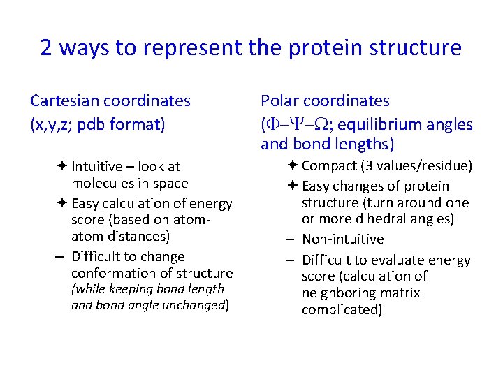
2 ways to represent the protein structure Cartesian coordinates (x, y, z; pdb format) Intuitive – look at molecules in space Easy calculation of energy score (based on atom distances) – Difficult to change conformation of structure (while keeping bond length and bond angle unchanged) Polar coordinates (F-Y-W; equilibrium angles and bond lengths) Compact (3 values/residue) Easy changes of protein structure (turn around one or more dihedral angles) – Non-intuitive – Difficult to evaluate energy score (calculation of neighboring matrix complicated)

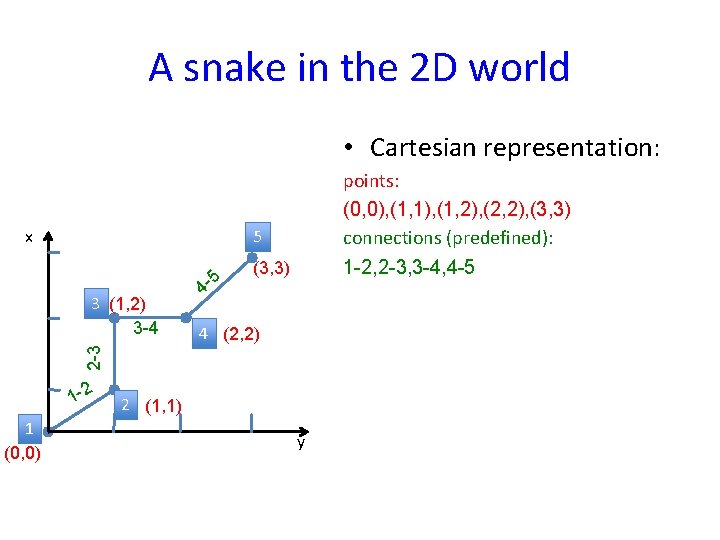
A snake in the 2 D world • Cartesian representation: x points: (0, 0), (1, 1), (1, 2), (2, 2), (3, 3) connections (predefined): 1 -2, 2 -3, 3 -4, 4 -5 5 (3, 3) 4 (2, 2) 2 -3 3 (1, 2) 3 -4 5 4 - 1 -2 1 (0, 0) 2 (1, 1) y

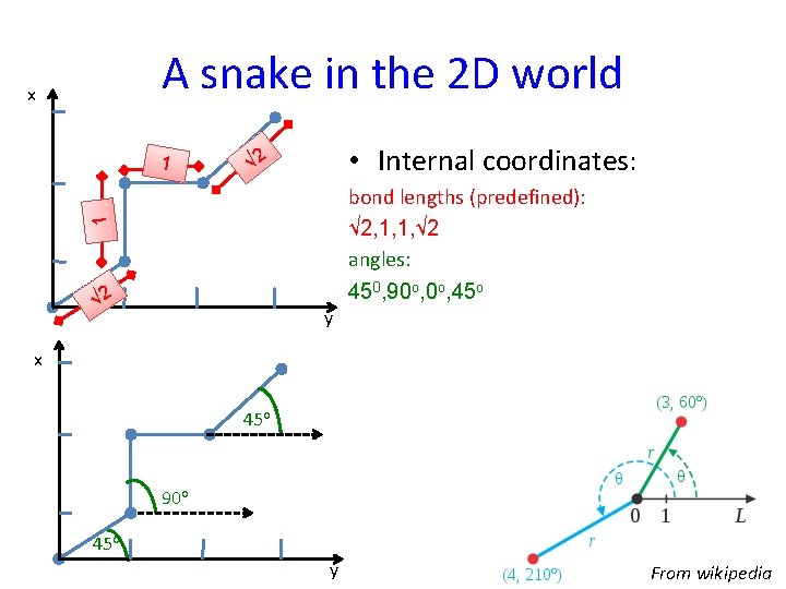
A snake in the 2 D world x 1 • Internal coordinates: √ 2 1 bond lengths (predefined): √ 2, 1, 1, √ 2 angles: 450, 90 o, 45 o √ 2 y x 45 o 90 o 45 o y From wikipedia

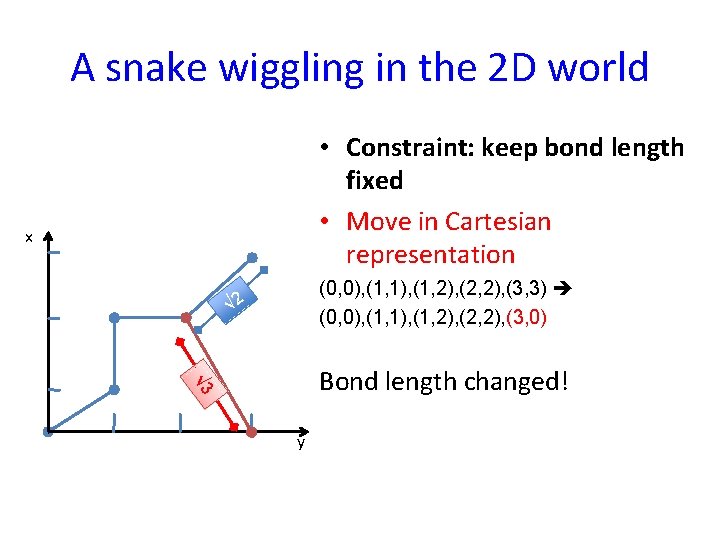
A snake wiggling in the 2 D world • Constraint: keep bond length fixed • Move in Cartesian representation x (0, 0), (1, 1), (1, 2), (2, 2), (3, 3) (0, 0), (1, 1), (1, 2), (2, 2), (3, 0) √ 2 √ 3 Bond length changed! y

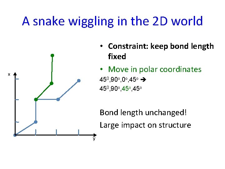
A snake wiggling in the 2 D world • Constraint: keep bond length fixed • Move in polar coordinates x 450, 90 o, 45 o Bond length unchanged! Large impact on structure y

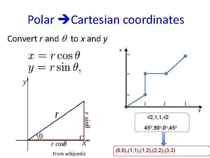
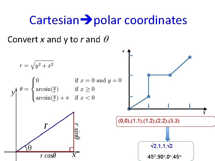
Polar Cartesian coordinates Convert r and q to x and y x y √ 2, 1, 1, √ 2 450, 90 o, 45 o From wikipedia (0, 0), (1, 1), (1, 2), (2, 2), (3, 3)

Cartesian polar coordinates Convert x and y to r and q x y (0, 0), (1, 1), (1, 2), (2, 2), (3, 3) √ 2, 1, 1, √ 2 450, 90 o, 45 o

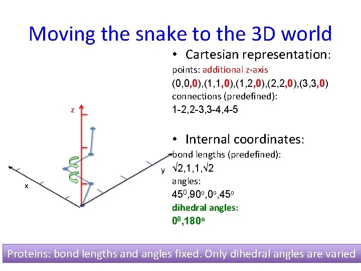
Moving the snake to the 3 D world • Cartesian representation: z points: additional z-axis (0, 0, 0), (1, 1, 0), (1, 2, 0), (2, 2, 0), (3, 3, 0) connections (predefined): 1 -2, 2 -3, 3 -4, 4 -5 • Internal coordinates: x bond lengths (predefined): y √ 2, 1, 1, √ 2 angles: 450, 90 o, 45 o dihedral angles: 00, 180 o Proteins: bond lengths and angles fixed. Only dihedral angles are varied

Dihedral angles c 1 -c 4 define side chain • Dihedral angle: defines geometry of 4 consecutive atoms (given bond lengths and angles) From wikipedia

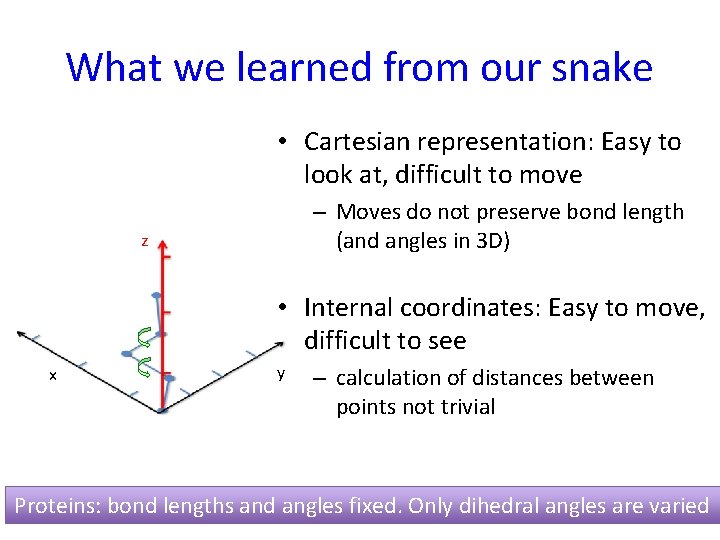
What we learned from our snake • Cartesian representation: Easy to look at, difficult to move – Moves do not preserve bond length (and angles in 3 D) z • Internal coordinates: Easy to move, difficult to see x y – calculation of distances between points not trivial Proteins: bond lengths and angles fixed. Only dihedral angles are varied

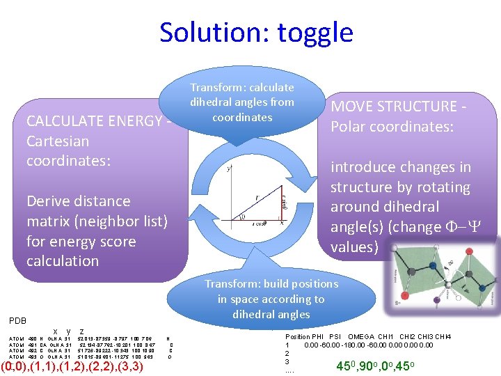
Solution: toggle CALCULATE ENERGY Cartesian coordinates: Derive distance matrix (neighbor list) for energy score calculation MOVE STRUCTURE Polar coordinates: introduce changes in structure by rotating around dihedral angle(s) (change F-Y values) Transform: build positions in space according to dihedral angles PDB x ATOM …. Transform: calculate dihedral angles from coordinates 490 491 492 493 y N GLN A 31 CA GLN A 31 C GLN A 31 O GLN A 31 z 52. 013 -87. 359 -8. 797 1. 00 7. 06 52. 134 -87. 762 -10. 201 1. 00 8. 67 51. 726 -89. 222 -10. 343 1. 00 10. 90 51. 015 -89. 601 -11. 275 1. 00 9. 63 (0, 0), (1, 1), (1, 2), (2, 2), (3, 3) N C C O Position PHI PSI OMEGA CHI 1 CHI 2 CHI 3 CHI 4 1 0. 00 -60. 00 -180. 00 -60. 00 2 3 0 o o o …. 45 , 90 , 45

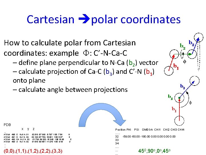
Cartesian polar coordinates How to calculate polar from Cartesian coordinates: example F: C’-N-Ca-C – define plane perpendicular to N-Ca (b 2) vector – calculate projection of Ca-C (b 3) and C’-N (b 1) onto plane – calculate angle between projections PDB x … ATOM …. 490 491 492 493 y C GLN A 31 N GLY A 32 CA GLY A 32 O GLY A 32 z 52. 013 -87. 359 -8. 797 1. 00 7. 06 52. 134 -87. 762 -10. 201 1. 00 8. 67 51. 726 -89. 222 -10. 343 1. 00 10. 90 51. 015 -89. 601 -11. 275 1. 00 9. 63 (0, 0), (1, 1), (1, 2), (2, 2), (3, 3) N C C O Position PHI PSI OMEGA CHI 1 CHI 2 CHI 3 CHI 4 …. . 32 -59. 00 -60. 00 -180. 00 33 34 …. 0 o o o … … 45 , 90 , 45

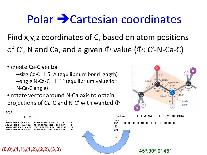
Polar Cartesian coordinates Find x, y, z coordinates of C, based on atom positions of C’, N and Ca, and a given F value (F: C’-N-Ca-C) • create Ca-C vector: –size Ca-C=1. 51 A (equilibrium bond length) –angle N-Ca-C= 111 o (equilibrium value for N-Ca-C angle) • rotate vector around N-Ca axis to obtain projections of Ca-C and N-C’ with wanted F PDB x … ATOM …. 490 491 492 493 y C GLN A 31 N GLY A 32 CA GLY A 32 O GLY A 32 z 52. 013 -87. 359 -8. 797 1. 00 7. 06 52. 134 -87. 762 -10. 201 1. 00 8. 67 51. 726 -89. 222 -10. 343 1. 00 10. 90 51. 015 -89. 601 -11. 275 1. 00 9. 63 (0, 0), (1, 1), (1, 2), (2, 2), (3, 3) N C C O Position PHI PSI OMEGA CHI 1 CHI 2 CHI 3 CHI 4 …. . 32 -59. 00 -60. 00 -180. 00 33 34 …. … … 450, 90 o, 45 o

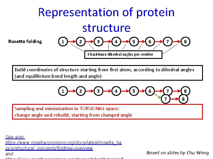
Representation of protein structure Rosetta folding 1 2 3 4 5 6 7 8 3 backbone dihedral angles per residue Build coordinates of structure starting from first atom, according to dihedral angles (and equilibrium bond length and angle) 1 2 3 4 5 6 7 7 8 8 Sampling and minimization in TORSIONAL space: change angle and rebuild, starting from changed angle See also: https: //www. rosettacommons. org/docs/latest/rosetta_ba sics/structural_concepts/foldtree-overview and Based on slides by Chu Wang

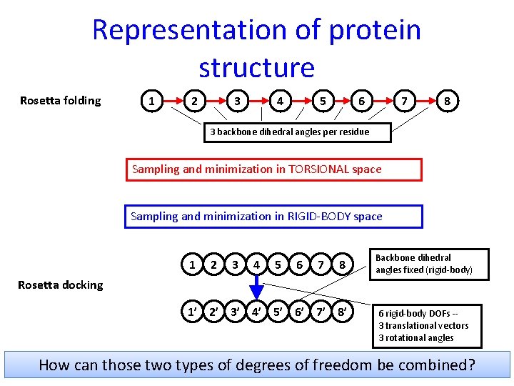
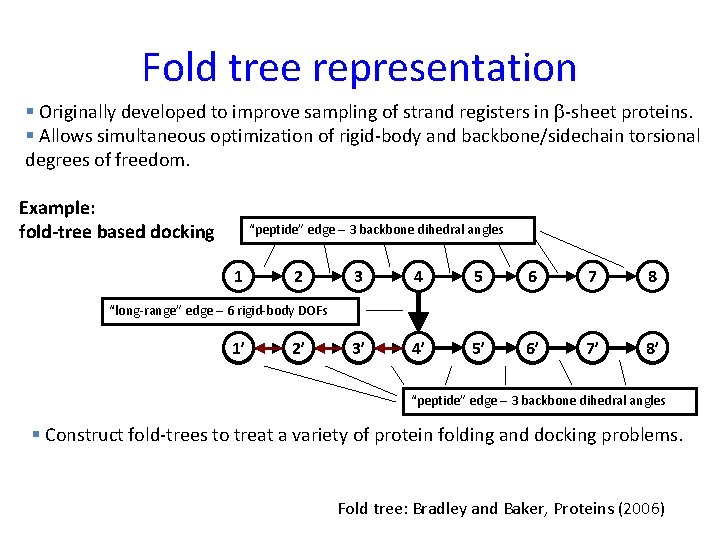
Representation of protein structure Rosetta folding 1 2 3 4 5 6 7 8 3 backbone dihedral angles per residue Sampling and minimization in TORSIONAL space Sampling and minimization in RIGID-BODY space 1 2 3 4 5 6 7 8 Backbone dihedral angles fixed (rigid-body) Rosetta docking 1’ 2’ 3’ 4’ 5’ 6’ 7’ 8’ 6 rigid-body DOFs -3 translational vectors 3 rotational angles How can those two types of degrees of freedom be combined?

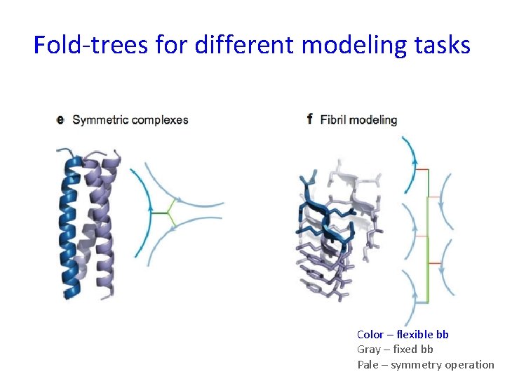
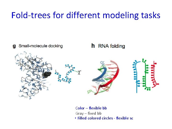
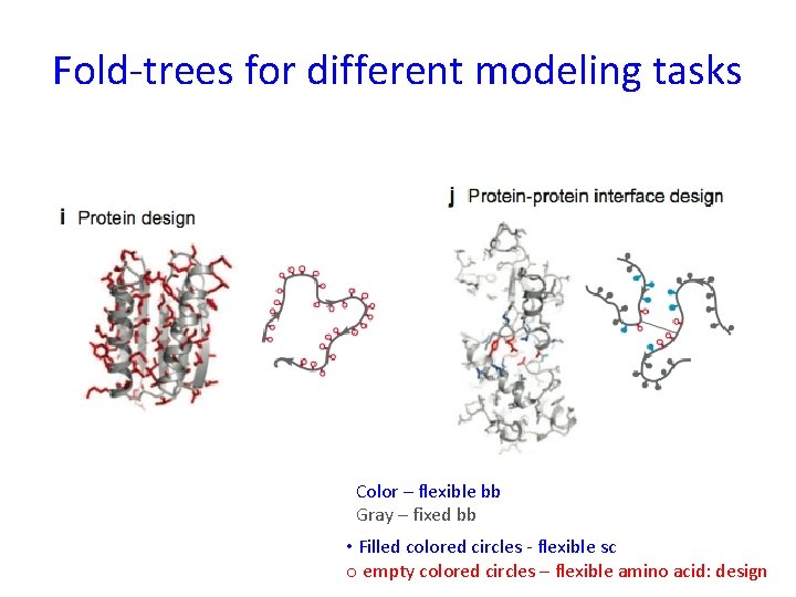
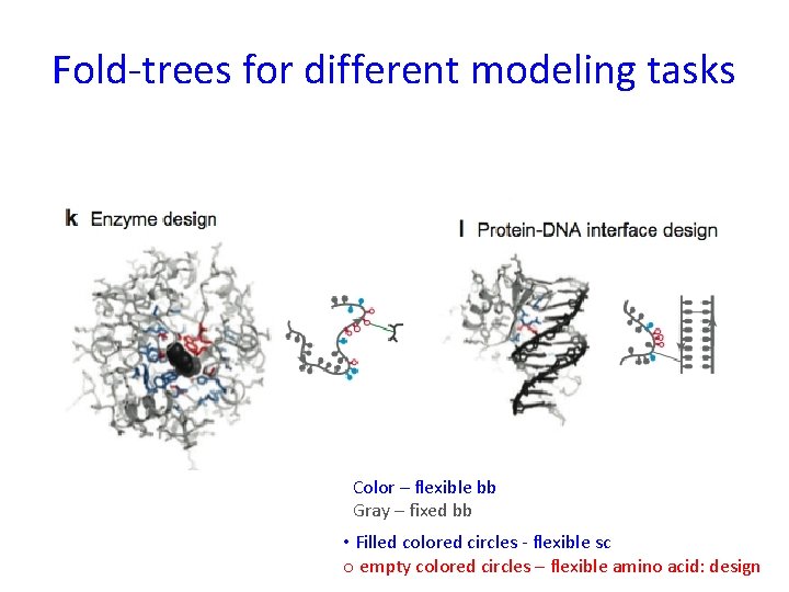
Fold tree representation § Originally developed to improve sampling of strand registers in -sheet proteins. § Allows simultaneous optimization of rigid-body and backbone/sidechain torsional degrees of freedom. Example: fold-tree based docking “peptide” edge – 3 backbone dihedral angles 1 2 3 4 5 6 7 8 3’ 4’ 5’ 6’ 7’ 8’ “long-range” edge – 6 rigid-body DOFs 1’ 2’ “peptide” edge – 3 backbone dihedral angles § Construct fold-trees to treat a variety of protein folding and docking problems. Fold tree: Bradley and Baker, Proteins (2006)

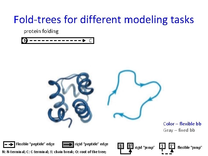
Fold-trees for different modeling tasks protein folding N C Color – flexible bb Gray – fixed bb Flexible “peptide” edge rigid “peptide” edge N: N-terminal; C: C-terminal; X: chain break; O: root of the tree; 1 1’ rigid “jump” 1 1’ flexible “jump”

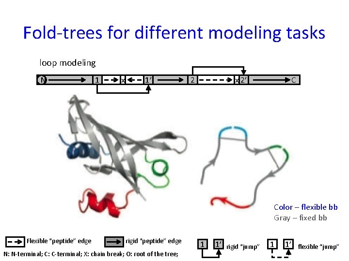
Fold-trees for different modeling tasks loop modeling N 1 x 1’ 2 x 2’ C Color – flexible bb Gray – fixed bb Flexible “peptide” edge rigid “peptide” edge N: N-terminal; C: C-terminal; X: chain break; O: root of the tree; 1 1’ rigid “jump” 1 1’ flexible “jump”

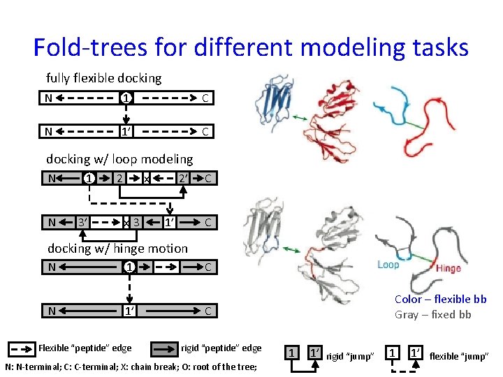
Fold-trees for different modeling tasks fully flexible docking N 1 C N 1’ C docking w/ loop modeling N N 1 3’ 2 x x 3 2’ 1’ C C docking w/ hinge motion N N 1 1’ Flexible “peptide” edge C Color – flexible bb Gray – fixed bb C rigid “peptide” edge N: N-terminal; C: C-terminal; X: chain break; O: root of the tree; 1 1’ rigid “jump” 1 1’ flexible “jump”

Fold-trees for different modeling tasks Color – flexible bb Gray – fixed bb Pale – symmetry operation

Fold-trees for different modeling tasks Color – flexible bb Gray – fixed bb • Filled colored circles - flexible sc

Fold-trees for different modeling tasks Color – flexible bb Gray – fixed bb • Filled colored circles - flexible sc o empty colored circles – flexible amino acid: design

Fold-trees for different modeling tasks Color – flexible bb Gray – fixed bb • Filled colored circles - flexible sc o empty colored circles – flexible amino acid: design

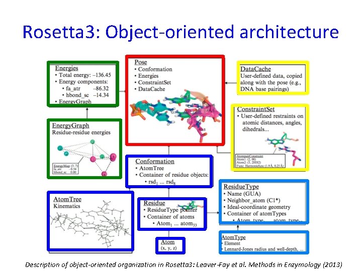
Rosetta 3: Object-oriented architecture Color – flexible bb Gray – fixed bb Description of object-oriented organization in Rosetta 3: Leaver-Fay et al. Methods in Enzymology (2013)