2 Fixed Effects Models 2 1 Basic fixedeffects

2. • • • Fixed Effects Models 2. 1 Basic fixed-effects model 2. 2 Exploring panel data 2. 3 Estimation and inference 2. 4 Model specification and diagnostics 2. 5 Model extensions Appendix 2 A - Least squares estimation

2. 1 Basic fixed effects model • Basic Elements • Subject i is observed on Ti occasions; – i = 1, . . . , n, – Ti T, the maximal number of time periods. • The response of interest is yit. • The K explanatory variables are xit = {xit 1, xit 2, . . . , xit. K}´, a vector of dimension K 1. • The population parameters are = ( 1, . . . , K)´, a vector of dimension K 1.

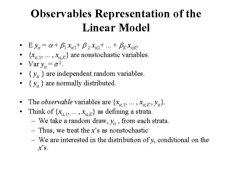
Observables Representation of the Linear Model • • • E yit = + 1 xit 1+ 2 xit 2+. . . + K xit. K. {xit, 1, . . . , xit, K} are nonstochastic variables. Var yit = σ 2. { yit } are independent random variables. { yit } are normally distributed. • The observable variables are {xit, 1, . . . , xit, K , yit}. • Think of {xit, 1, . . . , xit, K} as defining a strata. – We take a random draw, yit , from each strata. – Thus, we treat the x’s as nonstochastic – We are interested in the distribution of y, conditional on the x’s.

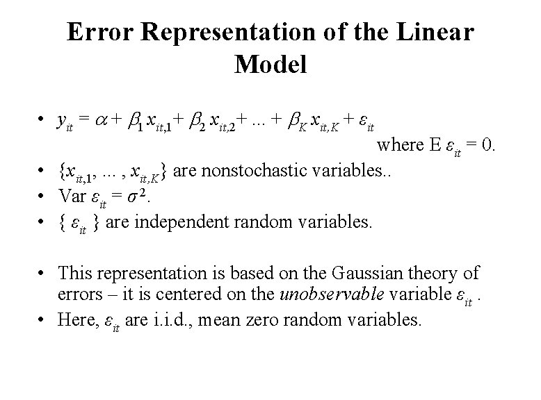
Error Representation of the Linear Model • yit = + 1 xit, 1+ 2 xit, 2+. . . + K xit, K + εit where E εit = 0. • {xit, 1, . . . , xit, K} are nonstochastic variables. . • Var εit = σ 2. • { εit } are independent random variables. • This representation is based on the Gaussian theory of errors – it is centered on the unobservable variable εit. • Here, εit are i. i. d. , mean zero random variables.

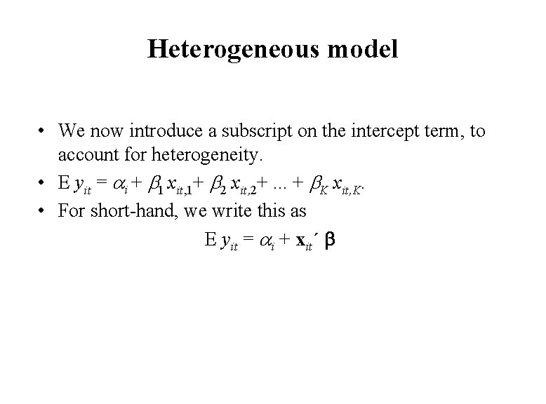
Heterogeneous model • We now introduce a subscript on the intercept term, to account for heterogeneity. • E yit = i + 1 xit, 1+ 2 xit, 2+. . . + K xit, K. • For short-hand, we write this as E yit = i + xit´

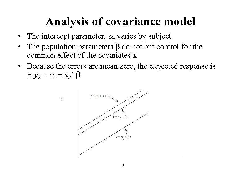
Analysis of covariance model • The intercept parameter, , varies by subject. • The population parameters do not but control for the common effect of the covariates x. • Because the errors are mean zero, the expected response is E yit = i + xit´ .

Parameters of interest • The common effects of the explanatory variables are dictated by the sign and magnitude of the betas ( ´s) – These are the parameters of interest • The intercept parameters vary by subject and account for different behavior of subjects. – The intercept parameters control for the heterogeneity of subjects. – Because they are of secondary interest, the intercepts are called nuisance parameters.

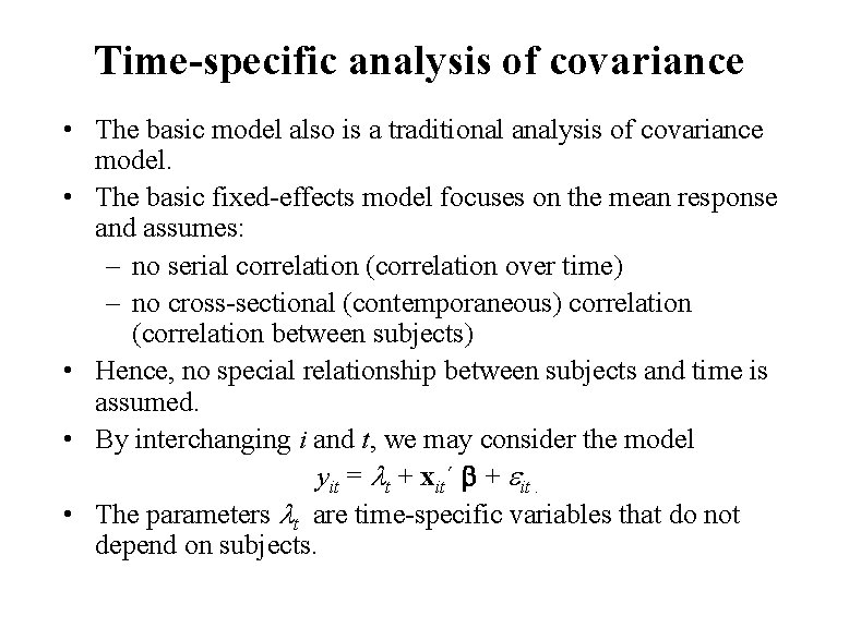
Time-specific analysis of covariance • The basic model also is a traditional analysis of covariance model. • The basic fixed-effects model focuses on the mean response and assumes: – no serial correlation (correlation over time) – no cross-sectional (contemporaneous) correlation (correlation between subjects) • Hence, no special relationship between subjects and time is assumed. • By interchanging i and t, we may consider the model yit = t + xit´ + it. • The parameters t are time-specific variables that do not depend on subjects.

Subject and time heterogeneity • Typically, the number of subjects, n, substantially exceeds the maximal number of time periods, T. • Typically, the heterogeneity among subjects explains a greater proportion of variability than the heterogeneity among time periods. • Thus, we begin with the “basic” model yit = i + xit´ + it. – This model allows explicit parameterization of the subject-specific heterogeneity. – By using binary variables for the time dimension, we can easily incorporate time-specific parameters.

2. 2 Exploring panel data • Why Explore? • Many important features of the data can be summarized numerically or graphically without reference to a model • Data exploration provides hints of the appropriate model – Many social science data sets are observational - they do not arise as the result of a designed experiment – The data collection mechanism does not dictate the model selection process. – To draw reliable inferences from the modeling procedure, it is important that the data be congruent with the model. • Exploring the data also alerts us to any unusual observations and/or subjects.

Data exploration techniques • • • Panel data is a special case of regression data. – Techniques applicable to regression are also useful for panel data. – Some commonly used techniques include: • Summarize the distribution of y and each x: – Graphically, through histograms and other density estimators – Numerically, through basic summary statistics (mean, median, standard deviation, minimum and maximum). • Summarize the relation between y and each x: – Graphically, through scatter plots – Numerically, through correlation statistics • Summary statistics by time period may be useful for detecting temporal patterns. Three more specialized (for panel data) techniques are: – Multiple time series plots – Scatterplots with symbols – Added variable plots. Section 2. 2 discusses additional techniques; these are performed after the fit of a preliminary model.

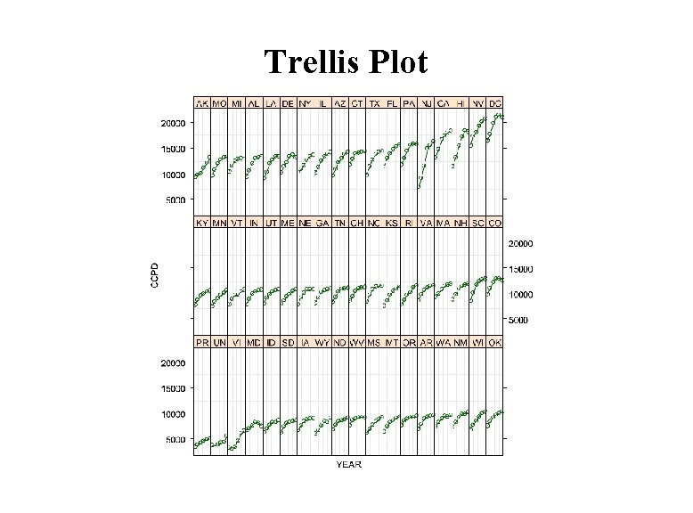
Multiple time series plots • Plot of the response, yit, versus time t. • Serially connect observations among common subjects. • This graph helps detect: – Patterns over time – Unusual observations and/or subjects. – Visualize the heterogeneity.

Scatterplots with symbols • Plot of the response, yit, versus an explanatory variable, xitj • Use a plotting symbol to encode the subject number “i” • See the relationship between the response and explanatory variable yet account for the varying intercepts. • Variation: If there is a separation in the x’s, such as increasing over time, – then we can serially connect the observations. – We do not need a separate plotting symbol for each subject.

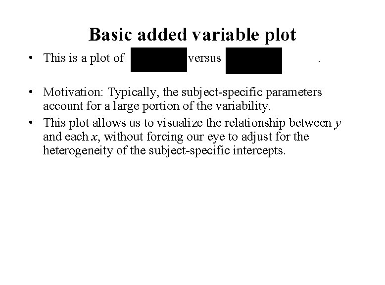
Basic added variable plot • This is a plot of versus . • Motivation: Typically, the subject-specific parameters account for a large portion of the variability. • This plot allows us to visualize the relationship between y and each x, without forcing our eye to adjust for the heterogeneity of the subject-specific intercepts.

Trellis Plot

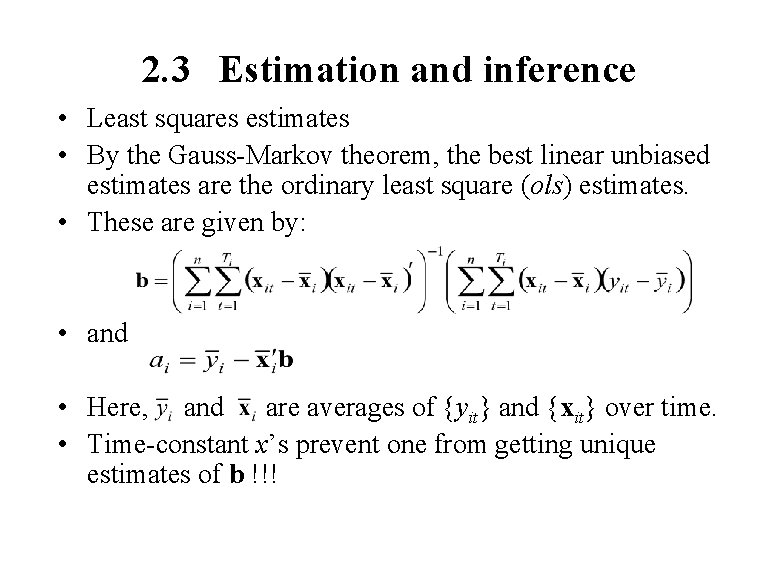
2. 3 Estimation and inference • Least squares estimates • By the Gauss-Markov theorem, the best linear unbiased estimates are the ordinary least square (ols) estimates. • These are given by: • and • Here, and are averages of {yit} and {xit} over time. • Time-constant x’s prevent one from getting unique estimates of b !!!

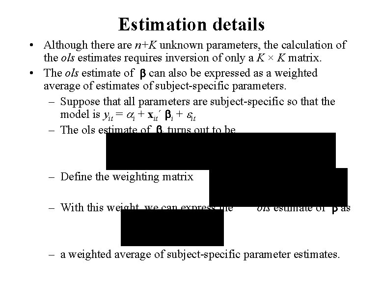
Estimation details • Although there are n+K unknown parameters, the calculation of the ols estimates requires inversion of only a K × K matrix. • The ols estimate of can also be expressed as a weighted average of estimates of subject-specific parameters. – Suppose that all parameters are subject-specific so that the model is yit = i + xit´ i + it – The ols estimate of i turns out to be – Define the weighting matrix – With this weight, we can express the ols estimate of as – a weighted average of subject-specific parameter estimates.

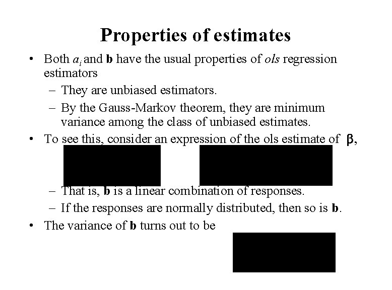
Properties of estimates • Both ai and b have the usual properties of ols regression estimators – They are unbiased estimators. – By the Gauss-Markov theorem, they are minimum variance among the class of unbiased estimates. • To see this, consider an expression of the ols estimate of , – That is, b is a linear combination of responses. – If the responses are normally distributed, then so is b. • The variance of b turns out to be

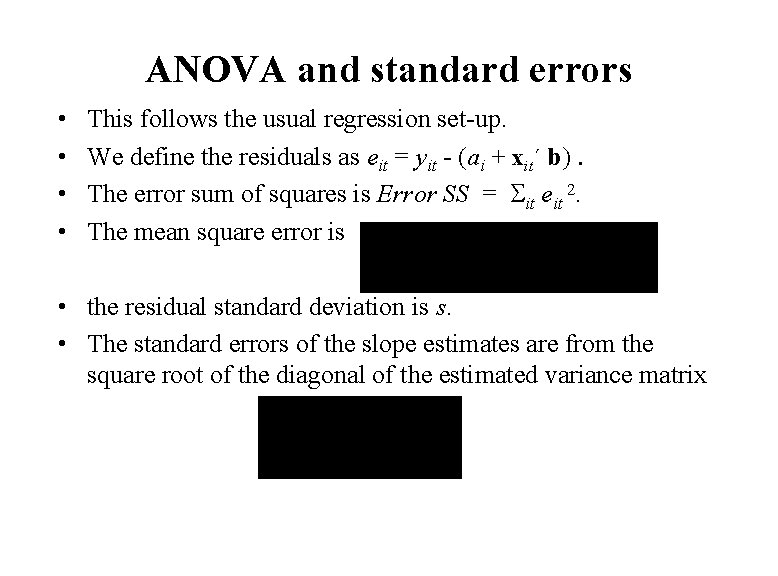
ANOVA and standard errors • • This follows the usual regression set-up. We define the residuals as eit = yit - (ai + xit´ b) The error sum of squares is Error SS = Sit eit 2. The mean square error is • the residual standard deviation is s. • The standard errors of the slope estimates are from the square root of the diagonal of the estimated variance matrix

Consistency of estimates • As the number of subjects (n) gets large, then b approaches . – Specifically, weak consistency means approaching (convergence) in probability. – This is a direct result of the unbiasedness and an assumption that Si Wi grows without bound. • As n gets large, the intercept estimates ai do not approach i. – They are inconsistent. – Intuitively, this is because we assume that the number of repeated measurements of i is Ti , a bounded number.

Other large sample approximations • Typically, the number of subjects is large relative to the number of time periods observed. • Thus, in deriving large sample approximations of the sampling distributions of estimators, assume that n although T remains fixed. • With this assumption, we have a central limit theorem for the slope estimator. – That is, b is approximately normally distributed even though responses are not. – The approximation improves as n becomes large. • Unlike the usual regression set-up, this is not true for the intercepts. If the responses are not normally distributed, then i are not even approximately normal.

2. 4 Model specification and diagnostics • • • Pooling Test Added variable plots Influence diagnostics Cross-sectional correlations Heteroscedasticity

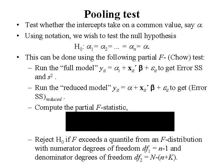
Pooling test • Test whether the intercepts take on a common value, say . • Using notation, we wish to test the null hypothesis H 0: 1= 2=. . . = n= • This can be done using the following partial F- (Chow) test: – Run the “full model” yit = i + xit´ + it to get Error SS and s 2. – Run the “reduced model” yit = + xit´ + it to get (Error SS)reduced. – Compute the partial F-statistic, – Reject H 0 if F exceeds a quantile from an F-distribution with numerator degrees of freedom df 1 = n-1 and denominator degrees of freedom df 2 = N-(n+K).

Added variable plot • An added variable plot (also called a partial regression plot) is a standard graphical device used in regression analysis • Purpose: To view the relationship between a response and an explanatory variable, after controlling for the linear effects of other explanatory variables. • Added variable plots allow us to visualize the relationship between y and each x, without forcing our eye to adjust for the differences induced by the other x’s. • The basic added variable plot is a special case.

Procedure for making an added variable plot • Select an explanatory variable, say xj. • Run a regression of y on the other explanatory variables (omitting xj) – calculate the residuals from this regression. Call these residuals e 1. • Run a regression of xj on the other explanatory variables (omitting xj) – calculate the residuals from this regression. Call these residuals e 2. • The plot of e 1 versus e 2 is an added variable plot.

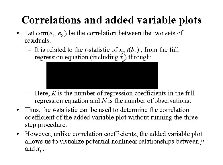
Correlations and added variable plots • Let corr(e 1, e 2 ) be the correlation between the two sets of residuals. – It is related to the t-statistic of xj, t(bj ) , from the full regression equation (including xj) through: – Here, K is the number of regression coefficients in the full regression equation and N is the number of observations. • Thus, the t-statistic can be used to determine the correlation coefficient of the added variable plot without running the three step procedure. • However, unlike correlation coefficients, the added variable plot allows us to visualize potential nonlinear relationships between y and xj.

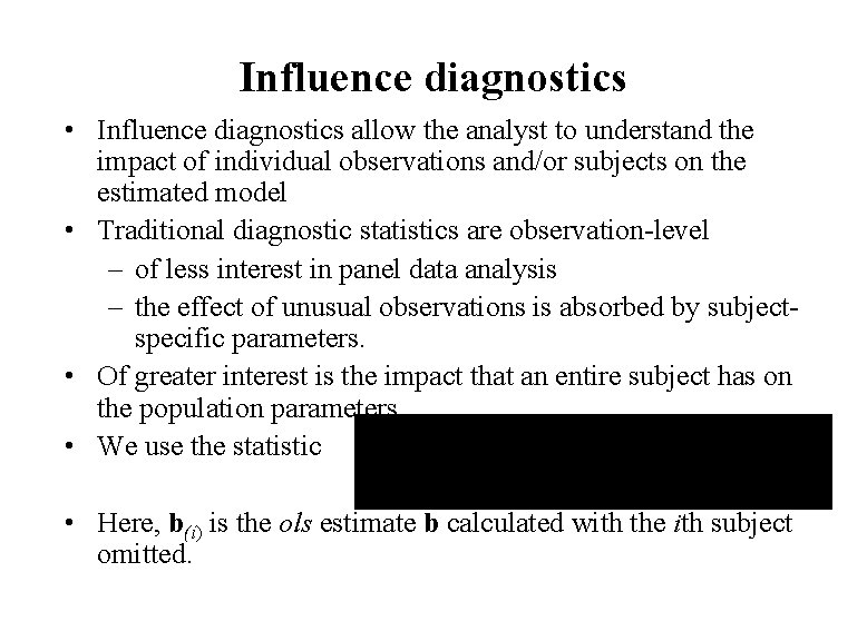
Influence diagnostics • Influence diagnostics allow the analyst to understand the impact of individual observations and/or subjects on the estimated model • Traditional diagnostic statistics are observation-level – of less interest in panel data analysis – the effect of unusual observations is absorbed by subjectspecific parameters. • Of greater interest is the impact that an entire subject has on the population parameters. • We use the statistic • Here, b(i) is the ols estimate b calculated with the ith subject omitted.

Calibration of influence diagnostic • The panel data influence diagnostic is similar to Cook’s distance for regression. – Cook’s distance is calculated at the observational level yet Bi(b) is at the subject level • The statistic Bi(b) has an approximate c 2 (chi-square) with K degrees of freedom – Observations with a “large” value of Bi(b) may be influential on the parameter estimates. – Use quantiles of the c 2 to quantify the adjective “large. ” • Influential observations warrant further investigation – they may need correction, additional variable specification to accommodate differences or deletion from the data set.

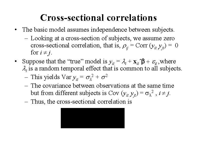
Cross-sectional correlations • The basic model assumes independence between subjects. – Looking at a cross-section of subjects, we assume zero cross-sectional correlation, that is, ij = Corr (yit , yjt) = 0 for i j. • Suppose that the “true” model is yit = t + xit´ + it , where t is a random temporal effect that is common to all subjects. – This yields Var yit = + – The covariance between observations at the same time but from different subjects is Cov (yit , yjt) = sl , i j. – Thus, the cross-sectional correlation is

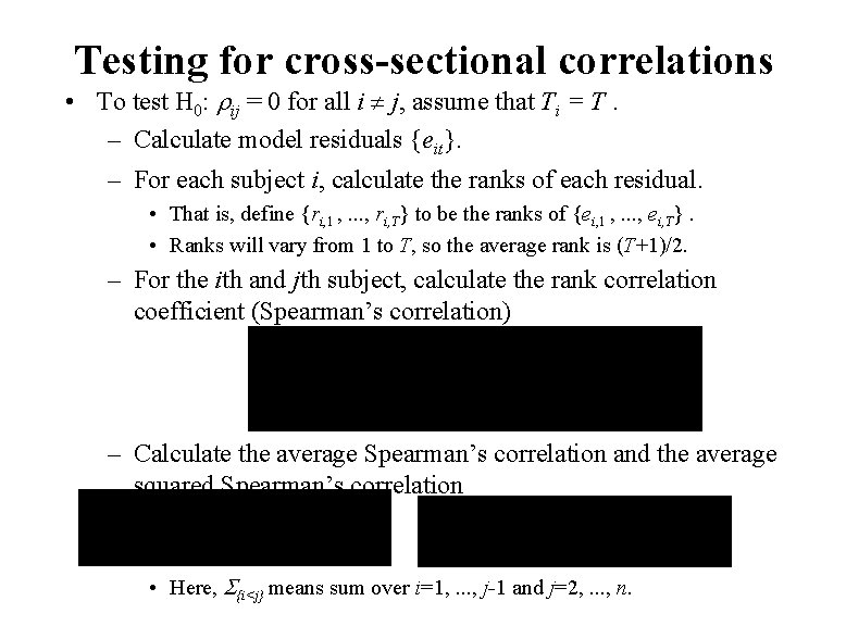
Testing for cross-sectional correlations • To test H 0: ij = 0 for all i j, assume that Ti = T. – Calculate model residuals {eit}. – For each subject i, calculate the ranks of each residual. • That is, define {ri, 1 , . . . , ri, T} to be the ranks of {ei, 1 , . . . , ei, T}. • Ranks will vary from 1 to T, so the average rank is (T+1)/2. – For the ith and jth subject, calculate the rank correlation coefficient (Spearman’s correlation) – Calculate the average Spearman’s correlation and the average squared Spearman’s correlation • Here, S{i<j} means sum over i=1, . . . , j-1 and j=2, . . . , n.

Calibration of cross-sectional correlation test • We compare R 2 ave to a distribution that is a weighted sum of chi-square random variables (Frees, 1995). • Specifically, define Q = a(T) (c 12 - (T-1)) + b(T) (c 22 - T(T-3)/2). – Here, c 12 and c 22 are independent chi-square random variables with T-1 and T(T-3)/2 degrees of freedom, respectively. – The constants are a(T) = 4(T+2) / (5(T-1)2(T+1)) and b(T) = 2(5 T+6) / (5 T(T-1)(T+1)).

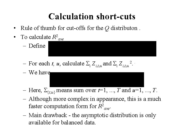
Calculation short-cuts • Rule of thumb for cut-offs for the Q distributon. • To calculate R 2 ave – Define – For each t, u, calculate Si Zi, t, u and Si Zi, t, u 2. . – We have – Here, S{t, u} means sum over t=1, . . . , T and u=1, . . . , T. – Although more complex in appearance, this is a much faster computation form for R 2 ave. – Main drawback - the asymptotic distribution is only available for balanced data.

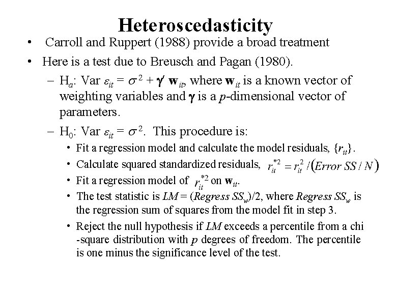
Heteroscedasticity • Carroll and Ruppert (1988) provide a broad treatment • Here is a test due to Breusch and Pagan (1980). – Ha: Var it = 2 + g¢ wit, where wit is a known vector of weighting variables and g is a p-dimensional vector of parameters. – H 0: Var it = 2. This procedure is: • • Fit a regression model and calculate the model residuals, {rit}. Calculate squared standardized residuals, Fit a regression model of on wit. The test statistic is LM = (Regress SSw)/2, where Regress SSw is the regression sum of squares from the model fit in step 3. • Reject the null hypothesis if LM exceeds a percentile from a chi -square distribution with p degrees of freedom. The percentile is one minus the significance level of the test.

2. 5 Model extensions • In panel data, subjects are measured repeatedly over time. Panel data analysis is useful for studying subject changes over time. • Repeated measurements of a subject tend to be intercorrelated. – Up to this point, we have used time-varying covariates to account for the presence of time in the mean response. – However, as in time series analysis, it is also useful to measure the tendencies in time patterns through a correlation structure.

Timing of observations • We now specify the time periods when the observations are made. – We assume that we have at most T observations on each subject. • These observations are made at time periods t 1, t 2, . . . , t. T. – Each subject has observations made at a subset of these T time periods, labeled t 1, t 2, . . . , t. Ti. – The subset may vary by subject and thus could be denoted by t 1 i, t 2 i, . . . , t. Tii. – For brevity, we use the simpler notation scheme and drop the second i subscript. • This framework, although notationally complex, allows for missing data and incomplete observations.

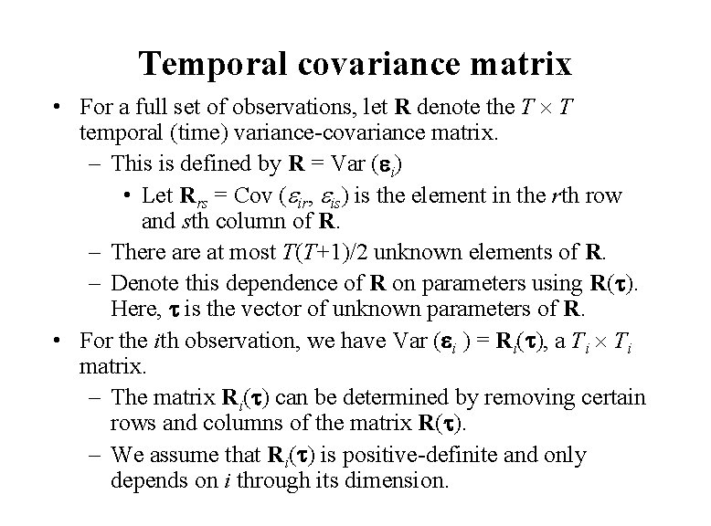
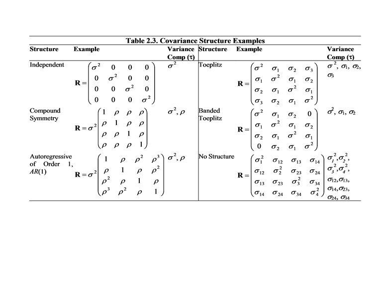
Temporal covariance matrix • For a full set of observations, let R denote the T T temporal (time) variance-covariance matrix. – This is defined by R = Var ( i) • Let Rrs = Cov ( ir, is) is the element in the rth row and sth column of R. – There at most T(T+1)/2 unknown elements of R. – Denote this dependence of R on parameters using R( ). Here, is the vector of unknown parameters of R. • For the ith observation, we have Var ( i ) = Ri( ), a Ti matrix. – The matrix Ri( ) can be determined by removing certain rows and columns of the matrix R( ). – We assume that Ri( ) is positive-definite and only depends on i through its dimension.

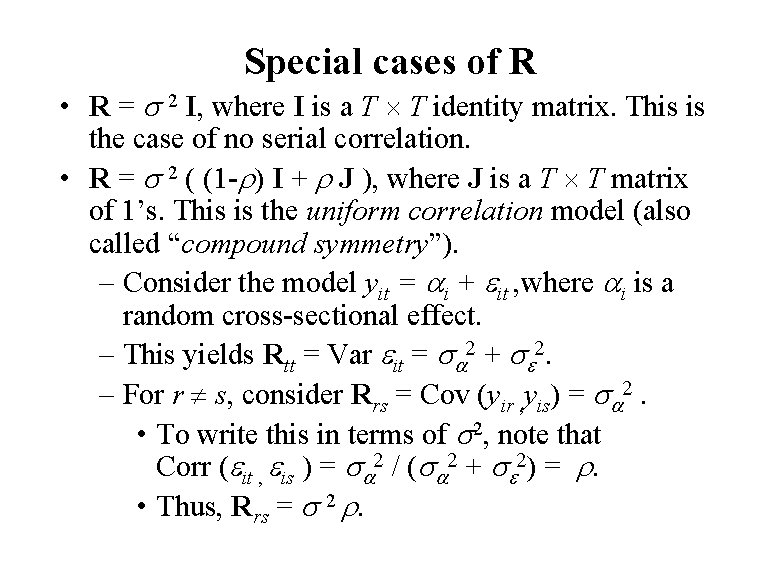
Special cases of R • R = 2 I, where I is a T T identity matrix. This is the case of no serial correlation. • R = 2 ( (1 - ) I + J ), where J is a T T matrix of 1’s. This is the uniform correlation model (also called “compound symmetry”). – Consider the model yit = i + it , where i is a random cross-sectional effect. – This yields Rtt = Var it = + . – For r s, consider Rrs = Cov (yir , yis) = . • To write this in terms of 2, note that Corr ( it , is ) = / ( + ) = • Thus, Rrs = 2 .

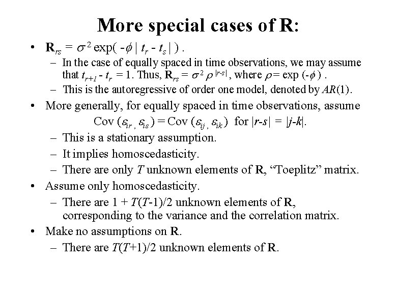
More special cases of R: • Rrs = 2 exp( - | tr - ts | ). – In the case of equally spaced in time observations, we may assume that tr+1 - tr = 1. Thus, Rrs = 2 |r-s| , where = exp (- ). – This is the autoregressive of order one model, denoted by AR(1). • More generally, for equally spaced in time observations, assume Cov ( ir , is ) = Cov ( ij , ik ) for |r-s| = |j-k|. – This is a stationary assumption. – It implies homoscedasticity. – There are only T unknown elements of R, “Toeplitz” matrix. • Assume only homoscedasticity. – There are 1 + T(T-1)/2 unknown elements of R, corresponding to the variance and the correlation matrix. • Make no assumptions on R. – There are T(T+1)/2 unknown elements of R.

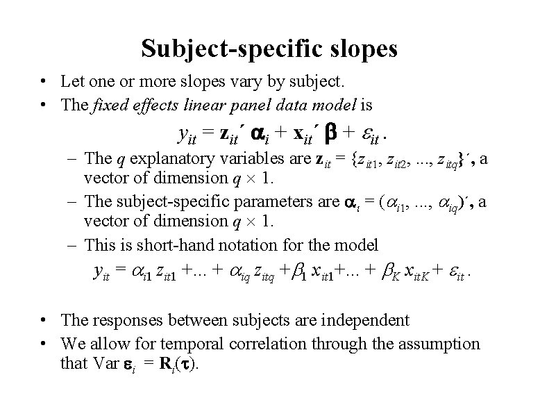
Subject-specific slopes • Let one or more slopes vary by subject. • The fixed effects linear panel data model is yit = zit´ i + xit´ + it. – The q explanatory variables are zit = {zit 1, zit 2, . . . , zitq}´, a vector of dimension q 1. – The subject-specific parameters are i = ( i 1, . . . , iq)´, a vector of dimension q 1. – This is short-hand notation for the model yit = i 1 zit 1 +. . . + iq zitq + 1 xit 1+. . . + K xit. K + it. • The responses between subjects are independent • We allow for temporal correlation through the assumption that Var i = Ri( ).

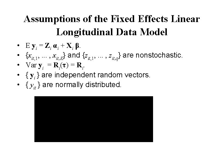
Assumptions of the Fixed Effects Linear Longitudinal Data Model • • • E yi = Zi αi + Xi β. {xit, 1, . . . , xit, K} and {zit, 1, . . . , zit, q} are nonstochastic. Var yi = Ri(τ) = Ri. { yi } are independent random vectors. { yit } are normally distributed.

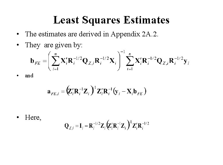
Least Squares Estimates • The estimates are derived in Appendix 2 A. 2. • They are given by: • and • Here,

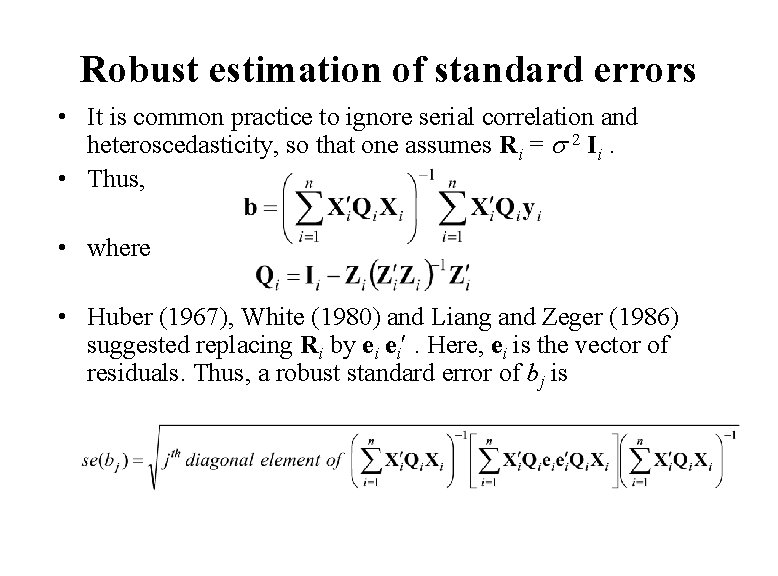
Robust estimation of standard errors • It is common practice to ignore serial correlation and heteroscedasticity, so that one assumes Ri = 2 Ii. • Thus, • where • Huber (1967), White (1980) and Liang and Zeger (1986) suggested replacing Ri by ei ei¢. Here, ei is the vector of residuals. Thus, a robust standard error of bj is