2 Derivatives Copyright Cengage Learning All rights reserved

2 Derivatives Copyright © Cengage Learning. All rights reserved.

2. 2 The Derivative as a Function Copyright © Cengage Learning. All rights reserved.

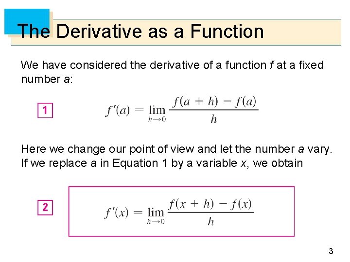
The Derivative as a Function We have considered the derivative of a function f at a fixed number a: Here we change our point of view and let the number a vary. If we replace a in Equation 1 by a variable x, we obtain 3

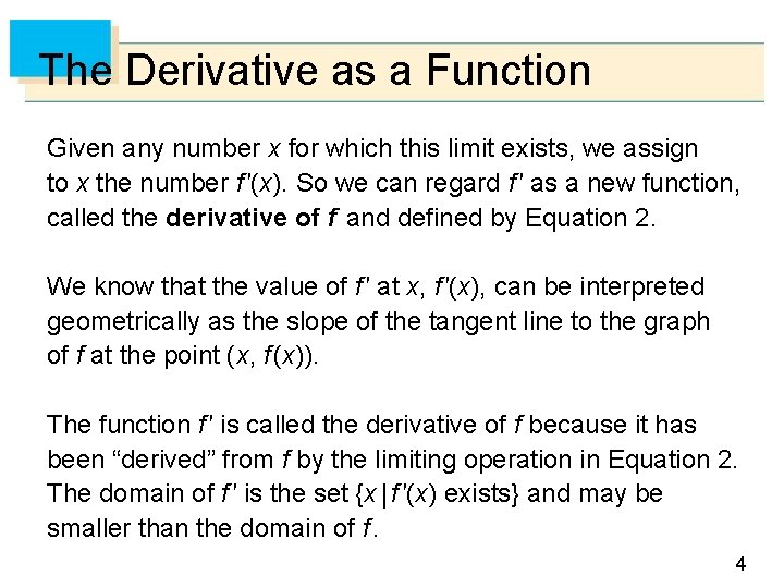
The Derivative as a Function Given any number x for which this limit exists, we assign to x the number f ′(x). So we can regard f ′ as a new function, called the derivative of f and defined by Equation 2. We know that the value of f ′ at x, f ′(x), can be interpreted geometrically as the slope of the tangent line to the graph of f at the point (x, f (x)). The function f ′ is called the derivative of f because it has been “derived” from f by the limiting operation in Equation 2. The domain of f ′ is the set {x | f ′(x) exists} and may be smaller than the domain of f. 4

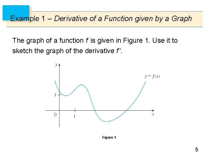
Example 1 – Derivative of a Function given by a Graph The graph of a function f is given in Figure 1. Use it to sketch the graph of the derivative f ′. Figure 1 5

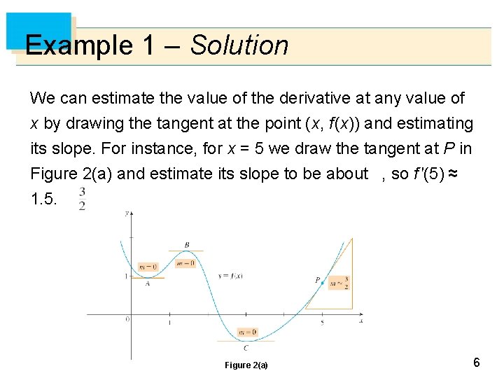
Example 1 – Solution We can estimate the value of the derivative at any value of x by drawing the tangent at the point (x, f (x)) and estimating its slope. For instance, for x = 5 we draw the tangent at P in Figure 2(a) and estimate its slope to be about , so f ′(5) ≈ 1. 5. Figure 2(a) 6

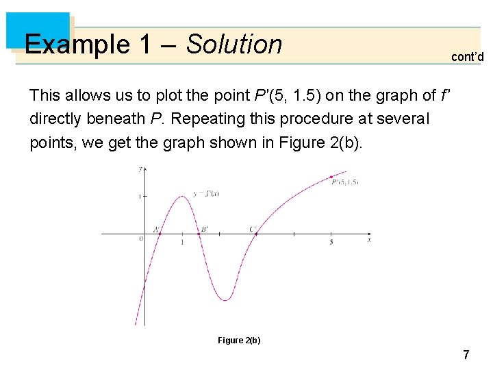
Example 1 – Solution cont’d This allows us to plot the point P ′(5, 1. 5) on the graph of f ′ directly beneath P. Repeating this procedure at several points, we get the graph shown in Figure 2(b) 7

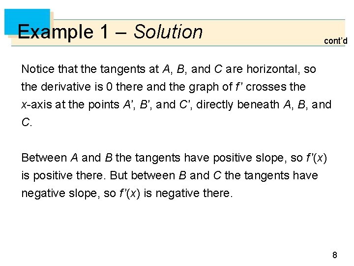
Example 1 – Solution cont’d Notice that the tangents at A, B, and C are horizontal, so the derivative is 0 there and the graph of f ′ crosses the x-axis at the points A′, B′, and C′, directly beneath A, B, and C. Between A and B the tangents have positive slope, so f ′(x) is positive there. But between B and C the tangents have negative slope, so f ′(x) is negative there. 8

Other Notations 9

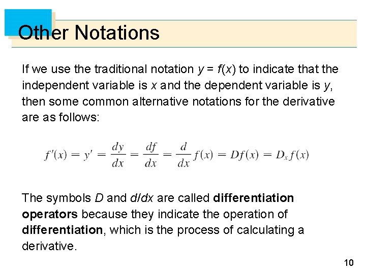
Other Notations If we use the traditional notation y = f (x) to indicate that the independent variable is x and the dependent variable is y, then some common alternative notations for the derivative are as follows: The symbols D and d/dx are called differentiation operators because they indicate the operation of differentiation, which is the process of calculating a derivative. 10

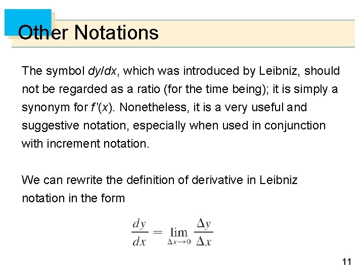
Other Notations The symbol dy/dx, which was introduced by Leibniz, should not be regarded as a ratio (for the time being); it is simply a synonym for f ′(x). Nonetheless, it is a very useful and suggestive notation, especially when used in conjunction with increment notation. We can rewrite the definition of derivative in Leibniz notation in the form 11

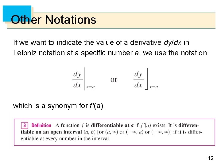
Other Notations If we want to indicate the value of a derivative dy/dx in Leibniz notation at a specific number a, we use the notation which is a synonym for f ′(a). 12

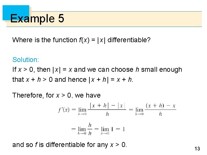
Example 5 Where is the function f (x) = | x | differentiable? Solution: If x > 0, then | x | = x and we can choose h small enough that x + h > 0 and hence | x + h | = x + h. Therefore, for x > 0, we have and so f is differentiable for any x > 0. 13

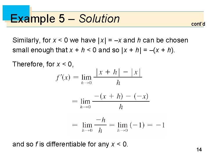
Example 5 – Solution cont’d Similarly, for x < 0 we have | x | = –x and h can be chosen small enough that x + h < 0 and so | x + h | = –(x + h). Therefore, for x < 0, and so f is differentiable for any x < 0. 14

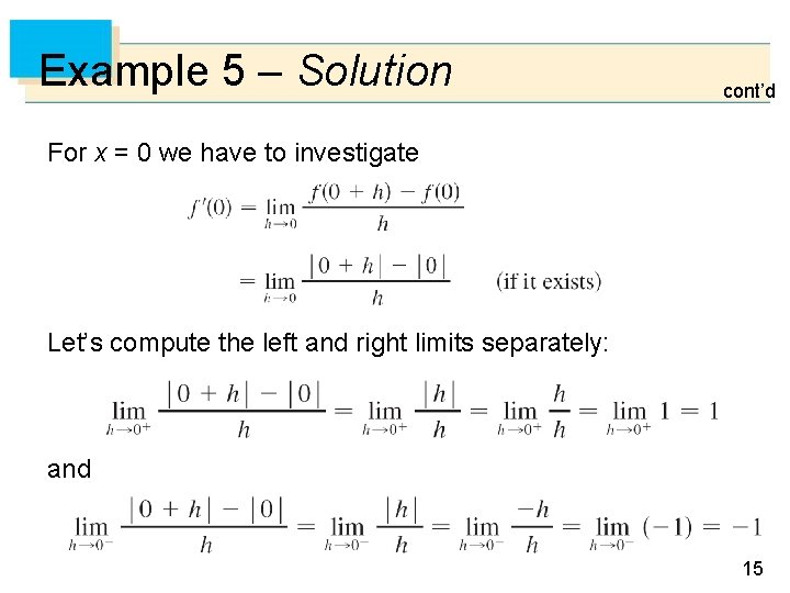
Example 5 – Solution cont’d For x = 0 we have to investigate Let’s compute the left and right limits separately: and 15

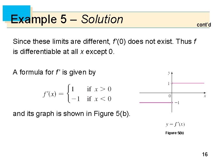
Example 5 – Solution cont’d Since these limits are different, f ′(0) does not exist. Thus f is differentiable at all x except 0. A formula for f ′ is given by and its graph is shown in Figure 5(b) 16

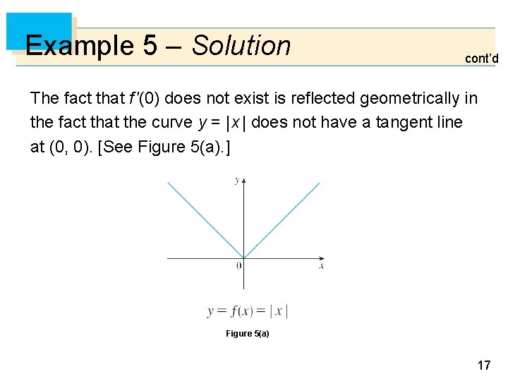
Example 5 – Solution cont’d The fact that f ′(0) does not exist is reflected geometrically in the fact that the curve y = | x | does not have a tangent line at (0, 0). [See Figure 5(a). ] Figure 5(a) 17

Other Notations Both continuity and differentiability are desirable properties for a function to have. The following theorem shows how these properties are related. The converse of Theorem 4 is false; that is, there are functions that are continuous but not differentiable. 18

How Can a Function Fail to Be Differentiable? 19

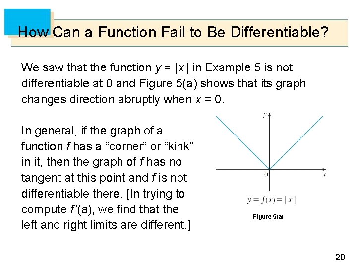
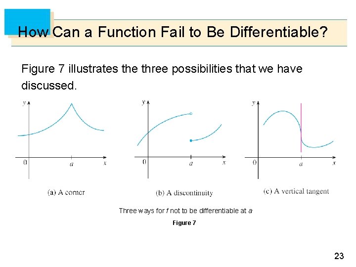
How Can a Function Fail to Be Differentiable? We saw that the function y = | x | in Example 5 is not differentiable at 0 and Figure 5(a) shows that its graph changes direction abruptly when x = 0. In general, if the graph of a function f has a “corner” or “kink” in it, then the graph of f has no tangent at this point and f is not differentiable there. [In trying to compute f ′(a), we find that the left and right limits are different. ] Figure 5(a) 20

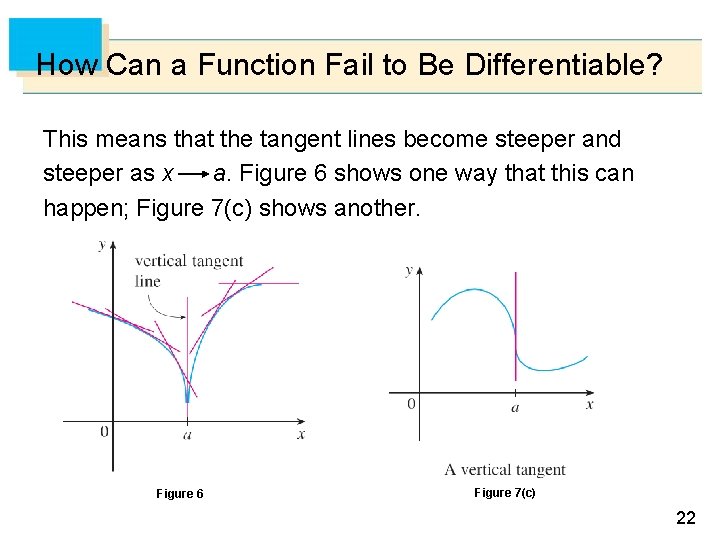
How Can a Function Fail to Be Differentiable? Theorem 4 gives another way for a function not to have a derivative. It says that if f is not continuous at a, then f is not differentiable at a. So at any discontinuity (for instance, a jump discontinuity) f fails to be differentiable. A third possibility is that the curve has a vertical tangent line when x = a; that is, f is continuous at a and 21

How Can a Function Fail to Be Differentiable? This means that the tangent lines become steeper and steeper as x a. Figure 6 shows one way that this can happen; Figure 7(c) shows another. Figure 6 Figure 7(c) 22

How Can a Function Fail to Be Differentiable? Figure 7 illustrates the three possibilities that we have discussed. Three ways for f not to be differentiable at a Figure 7 23

Higher Derivatives 24

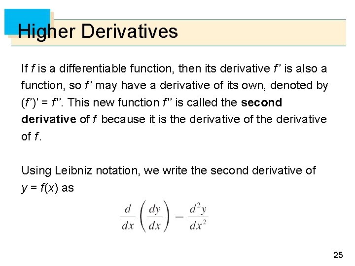
Higher Derivatives If f is a differentiable function, then its derivative f ′ is also a function, so f ′ may have a derivative of its own, denoted by (f ′)′ = f ′′. This new function f ′′ is called the second derivative of f because it is the derivative of f. Using Leibniz notation, we write the second derivative of y = f (x) as 25

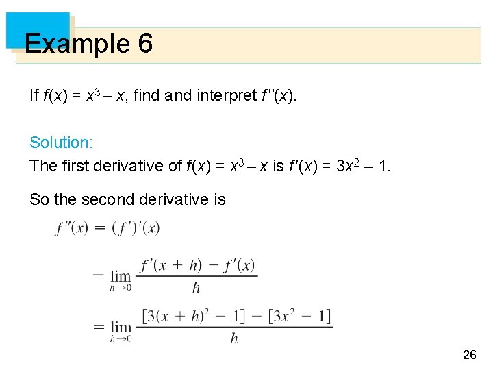
Example 6 If f (x) = x 3 – x, find and interpret f ′′(x). Solution: The first derivative of f (x) = x 3 – x is f ′(x) = 3 x 2 – 1. So the second derivative is 26

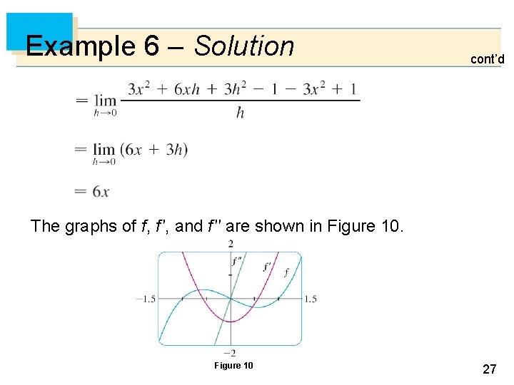
Example 6 – Solution cont’d The graphs of f, f ′, and f ′′ are shown in Figure 10 27

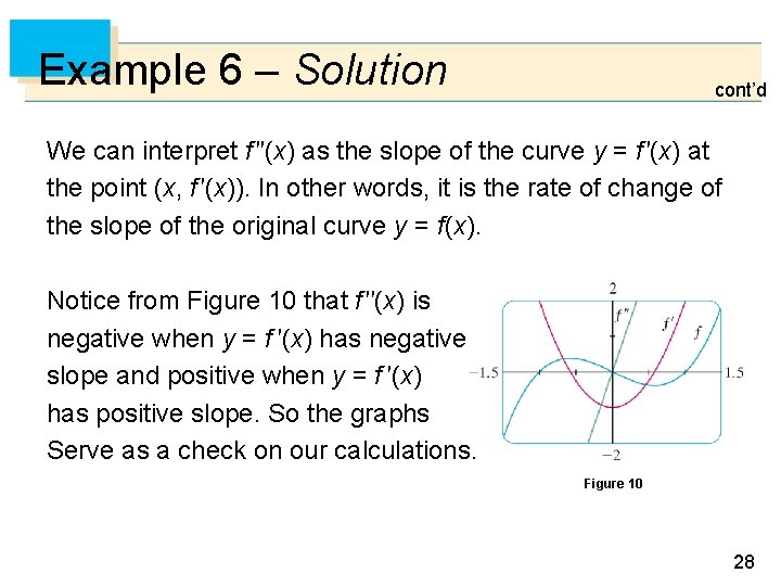
Example 6 – Solution cont’d We can interpret f ′′(x) as the slope of the curve y = f ′(x) at the point (x, f ′(x)). In other words, it is the rate of change of the slope of the original curve y = f (x). Notice from Figure 10 that f ′′(x) is negative when y = f ′(x) has negative slope and positive when y = f ′(x) has positive slope. So the graphs Serve as a check on our calculations. Figure 10 28

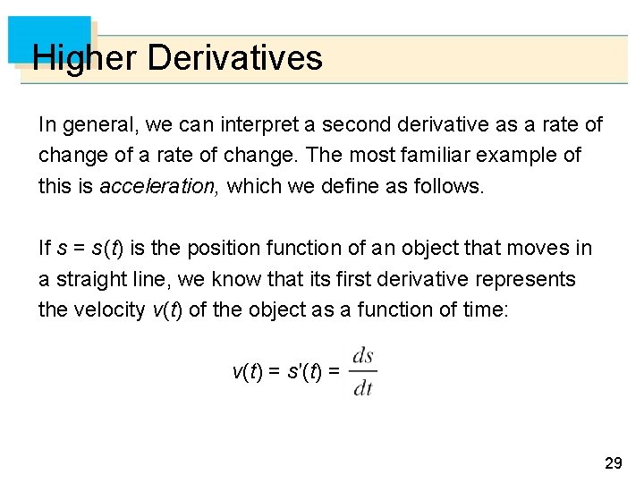
Higher Derivatives In general, we can interpret a second derivative as a rate of change of a rate of change. The most familiar example of this is acceleration, which we define as follows. If s = s (t) is the position function of an object that moves in a straight line, we know that its first derivative represents the velocity v(t) of the object as a function of time: v(t) = s′(t) = 29

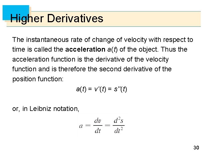
Higher Derivatives The instantaneous rate of change of velocity with respect to time is called the acceleration a(t) of the object. Thus the acceleration function is the derivative of the velocity function and is therefore the second derivative of the position function: a(t) = v ′(t) = s ′′(t) or, in Leibniz notation, 30

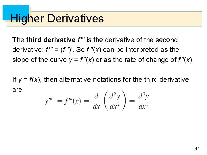
Higher Derivatives The third derivative f ′′′ is the derivative of the second derivative: f ′′′ = (f ′′)′. So f ′′′(x) can be interpreted as the slope of the curve y = f ′′(x) or as the rate of change of f ′′(x). If y = f (x), then alternative notations for the third derivative are 31

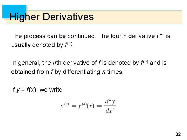
Higher Derivatives The process can be continued. The fourth derivative f ′′′′ is usually denoted by f (4). In general, the nth derivative of f is denoted by f (n) and is obtained from f by differentiating n times. If y = f (x), we write 32

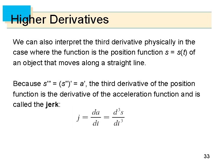
Higher Derivatives We can also interpret the third derivative physically in the case where the function is the position function s = s(t) of an object that moves along a straight line. Because s′′′ = (s′′)′ = a′, the third derivative of the position function is the derivative of the acceleration function and is called the jerk: 33

Higher Derivatives Thus the jerk j is the rate of change of acceleration. It is aptly named because a large jerk means a sudden change in acceleration, which causes an abrupt movement in a vehicle. 34