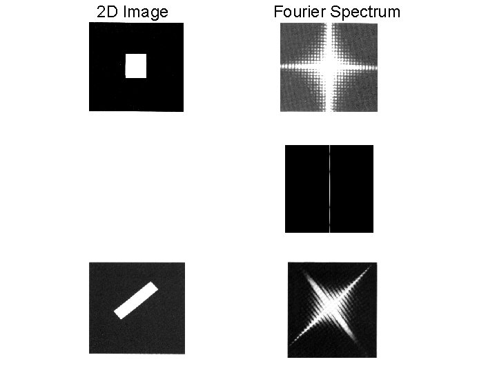
2 D Image Fourier Spectrum Fourier Transform Examples

2 D Image Fourier Spectrum

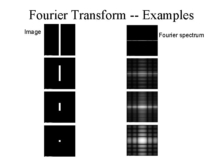
Fourier Transform -- Examples Image Fourier spectrum

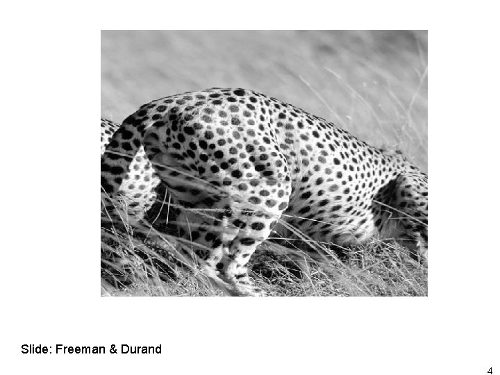
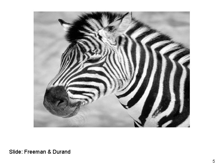
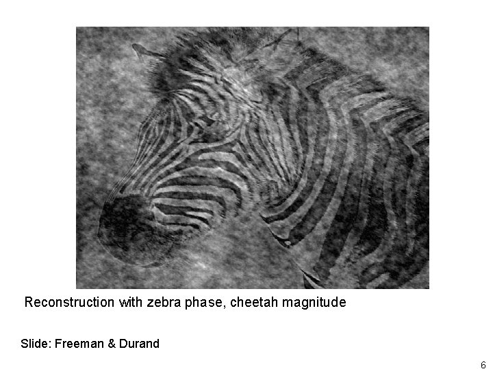
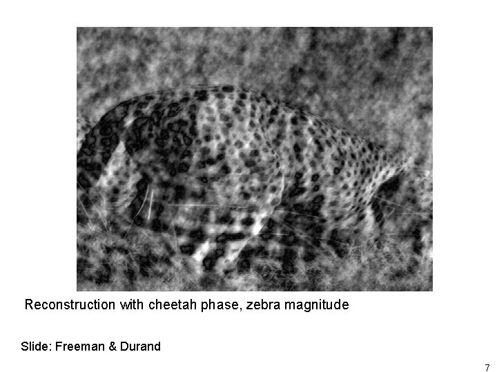
Phase and Magnitude • Curious fact All natural images have very similar magnitude transform. So why do they look different…? Phase in images matters a lot (more than magnitude) • Demonstration Take two pictures, swap the phase transforms, compute the inverse - what does the result look like? 3

Slide: Freeman & Durand 4

Slide: Freeman & Durand 5

Reconstruction with zebra phase, cheetah magnitude Slide: Freeman & Durand 6

Reconstruction with cheetah phase, zebra magnitude Slide: Freeman & Durand 7

Convolution

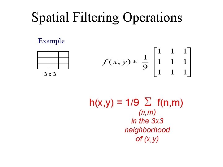
Spatial Filtering Operations Example 3 x 3 h(x, y) = 1/9 S f(n, m) in the 3 x 3 neighborhood of (x, y)

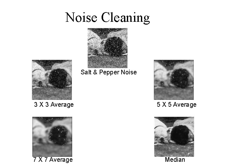
Noise Cleaning Salt & Pepper Noise 3 X 3 Average 5 X 5 Average 7 X 7 Average Median

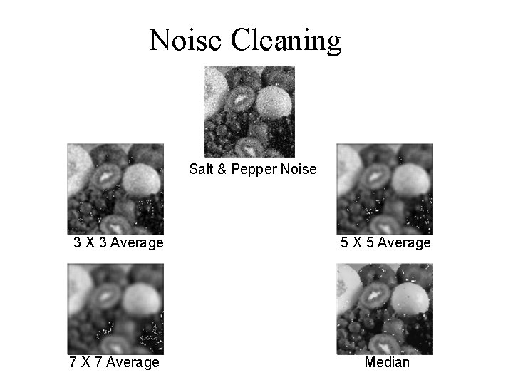
Noise Cleaning Salt & Pepper Noise 3 X 3 Average 5 X 5 Average 7 X 7 Average Median

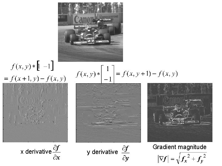
x derivative y derivative Gradient magnitude

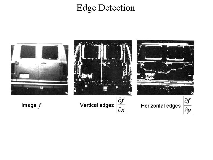
Edge Detection Image Vertical edges Horizontal edges

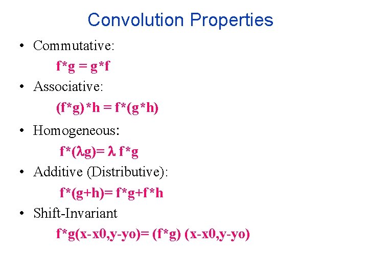
Convolution Properties • Commutative: f*g = g*f • Associative: (f*g)*h = f*(g*h) • Homogeneous: f*( g)= f*g • Additive (Distributive): f*(g+h)= f*g+f*h • Shift-Invariant f*g(x-x 0, y-yo)= (f*g) (x-x 0, y-yo)

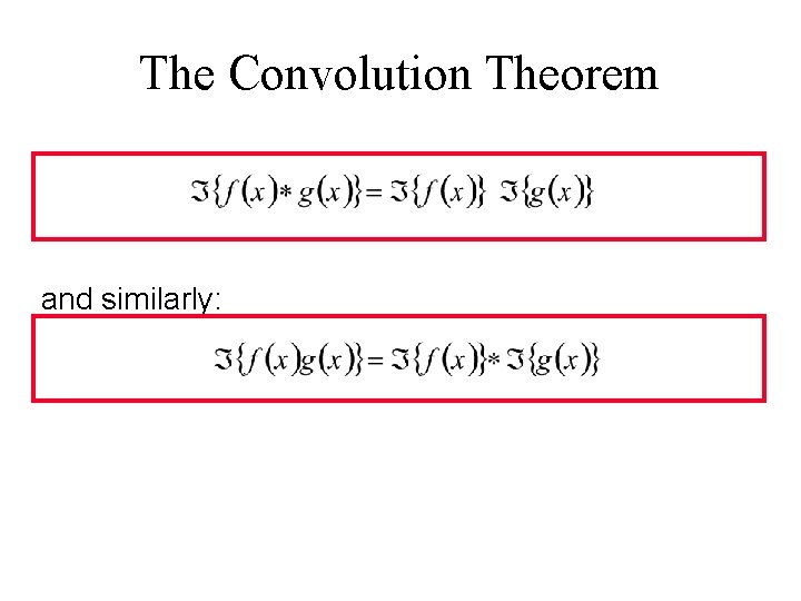
The Convolution Theorem and similarly:

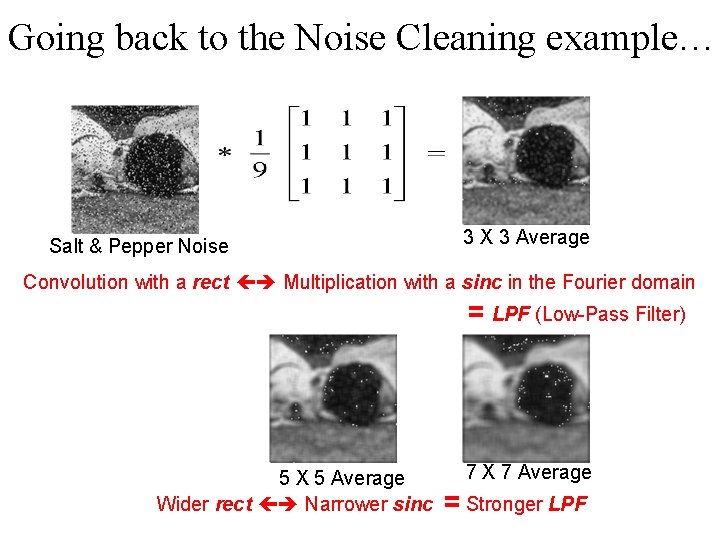
Going back to the Noise Cleaning example… Salt & Pepper Noise 3 X 3 Average Convolution with a rect Multiplication with a sinc in the Fourier domain = LPF (Low-Pass Filter) 5 X 5 Average Wider rect Narrower sinc 7 X 7 Average = Stronger LPF

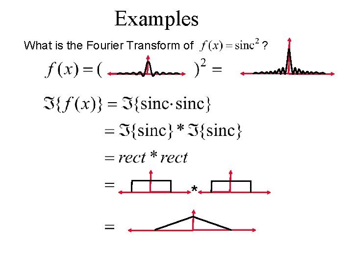
Examples What is the Fourier Transform of * ?

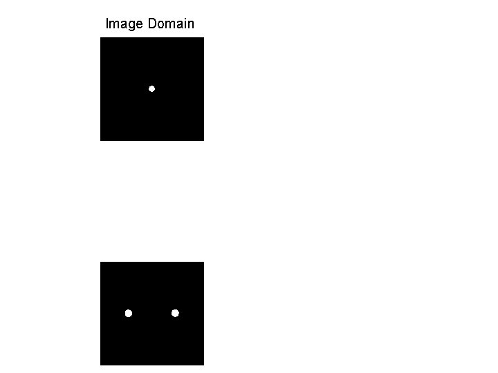
Image Domain Frequency Domain

The Sampling Theorem (developed on the board) Nyquist frequency, Aliasing, etc…

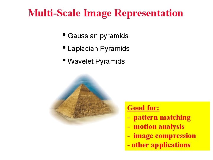
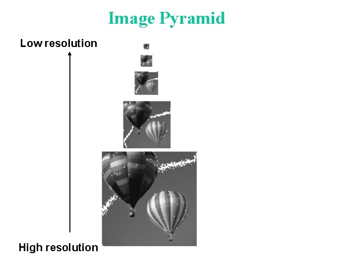
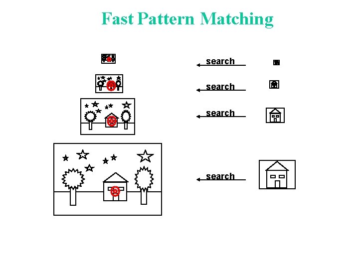
Multi-Scale Image Representation • Gaussian pyramids • Laplacian Pyramids • Wavelet Pyramids Good for: - pattern matching - motion analysis - image compression - other applications

Image Pyramid Low resolution High resolution

Fast Pattern Matching search

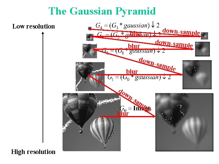
The Gaussian Pyramid Low resolution down-sample blur down-samp le blur down -sam ple blur do wn blur High resolution -sa mp le

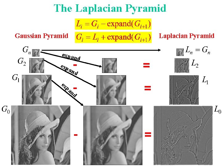
The Laplacian Pyramid Gaussian Pyramid expan - exp d and ex pa = - = nd

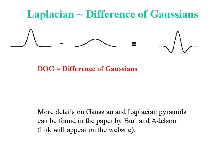
Laplacian ~ Difference of Gaussians - = DOG = Difference of Gaussians More details on Gaussian and Laplacian pyramids can be found in the paper by Burt and Adelson (link will appear on the website).

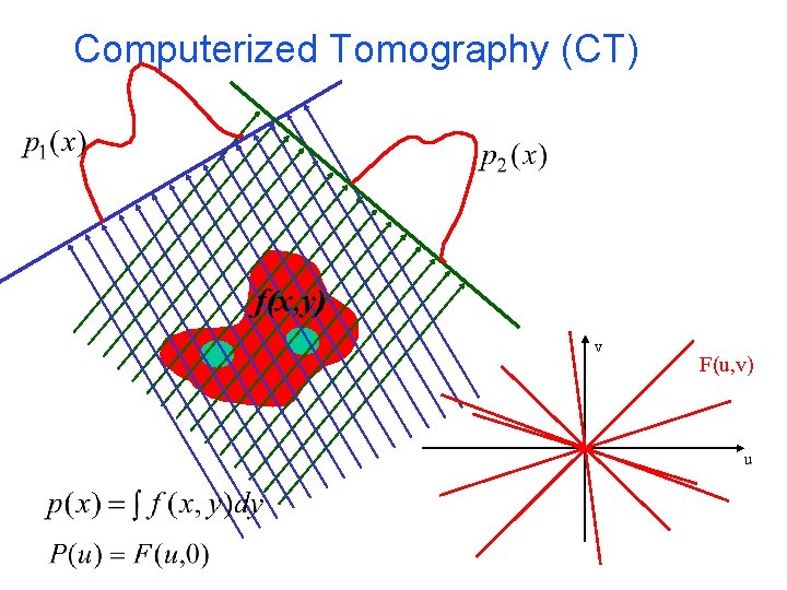
Computerized Tomography (CT) f(x, y) v F(u, v) u

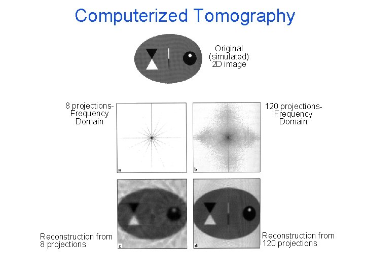
Computerized Tomography Original (simulated) 2 D image 8 projections. Frequency Domain Reconstruction from 8 projections 120 projections. Frequency Domain Reconstruction from 120 projections

End of Lesson. . . Exercise#1 -- will be posted on the website. (Theoretical exercise: To be done and submitted individually)