2 Consumers demand analysis Structure Factors influencing an

2. Consumer´s demand analysis

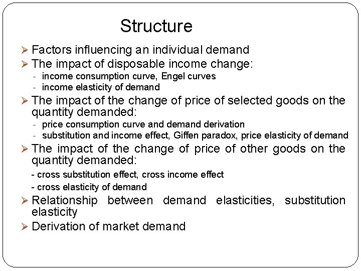
Structure Ø Factors influencing an individual demand Ø The impact of disposable income change: - income consumption curve, Engel curves - income elasticity of demand Ø The impact of the change of price of selected goods on the quantity demanded: - price consumption curve and demand derivation - substitution and income effect, Giffen paradox, price elasticity of demand Ø The impact of the change of price of other goods on the quantity demanded: - cross substitution effect, cross income effect - cross elasticity of demand Ø Relationship between demand elasticities, substitution elasticity Ø Derivation of market demand

Characteristics of an individual demand Individual demand = demand of the sole consumer. . . depends on: Ø disposable income Ø price of the selected goods Ø price of other goods Ø consumer´s preferences and expectations

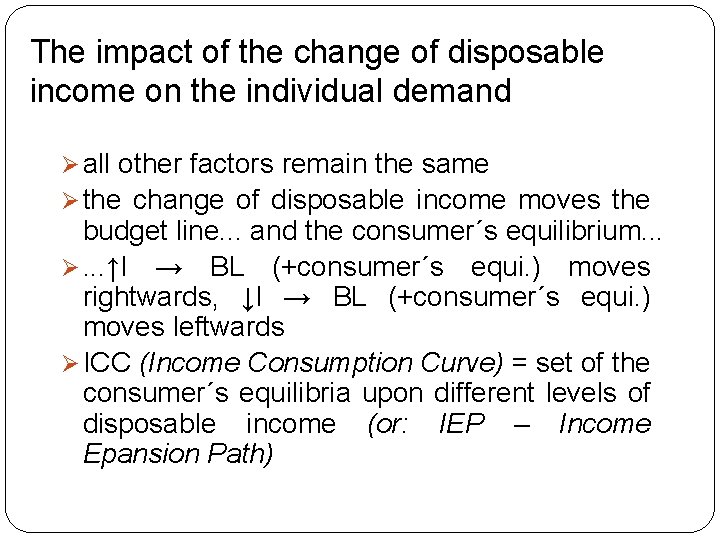
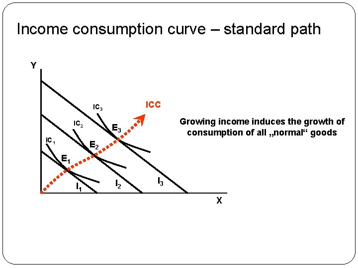
The impact of the change of disposable income on the individual demand Ø all other factors remain the same Ø the change of disposable income moves the budget line. . . and the consumer´s equilibrium. . . Ø. . . ↑I → BL (+consumer´s equi. ) moves rightwards, ↓I → BL (+consumer´s equi. ) moves leftwards Ø ICC (Income Consumption Curve) = set of the consumer´s equilibria upon different levels of disposable income (or: IEP – Income Epansion Path)

Income consumption curve – standard path Y ICC IC 3 IC 2 IC 1 Growing income induces the growth of consumption of all „normal“ goods E 3 E 2 E 1 I 2 I 3 X

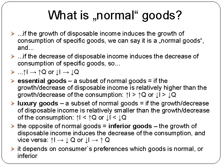
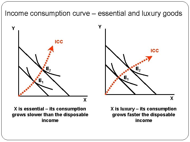
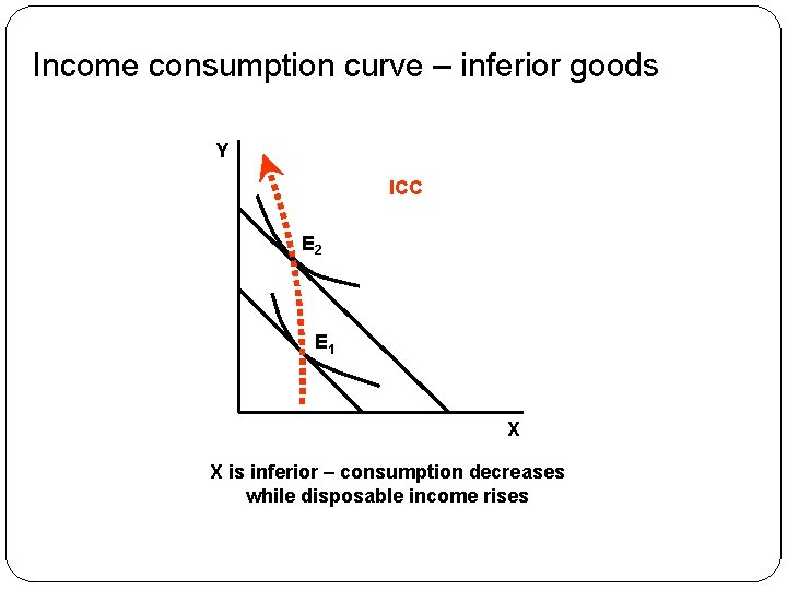
What is „normal“ goods? Ø. . . if the growth of disposable income induces the growth of Ø Ø Ø consumption of specific goods, we can say it is a „normal goods“, and. . . if the decrease of disposable income induces the decrease of consumption of specific goods, so. . . ↑I → ↑Q or ↓I → ↓Q essential goods – a subset of normal goods = if the growth/decrease of disposable income is relatively higher than the growth/decrease of the consumption: ↑I > ↑Q or ↓I > ↓Q luxury goods – a subset of normal goods = if the growth/decrease of disposable income is relatively smaller than the growth/decrease of the consumption: ↑I < ↑Q or ↓I < ↓Q the opposite of normal goods = inferior goods – the growth of disposable income induces the decrease of the consumption, and vice versa: ↑I → ↓ Q or ↓I → ↑ Q it depends on consumer´s preferences which goods is normal, or inferior

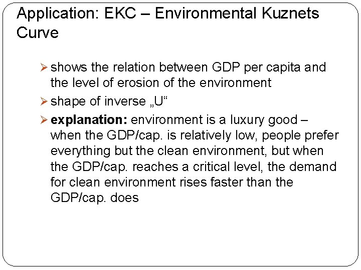
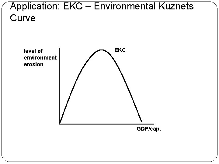
Application: EKC – Environmental Kuznets Curve Ø shows the relation between GDP per capita and the level of erosion of the environment Ø shape of inverse „U“ Ø explanation: environment is a luxury good – when the GDP/cap. is relatively low, people prefer everything but the clean environment, but when the GDP/cap. reaches a critical level, the demand for clean environment rises faster than the GDP/cap. does

Application: EKC – Environmental Kuznets Curve level of environment erosion EKC GDP/cap.

Income consumption curve – essential and luxury goods Y Y ICC E 2 E 1 X X is essential – its consumption grows slower than the disposable income X X is luxury – its consumption grows faster the disposable income

Income consumption curve – inferior goods Y ICC E 2 E 1 X X is inferior – consumption decreases while disposable income rises

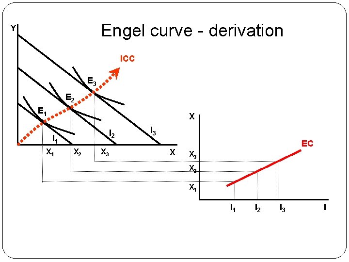
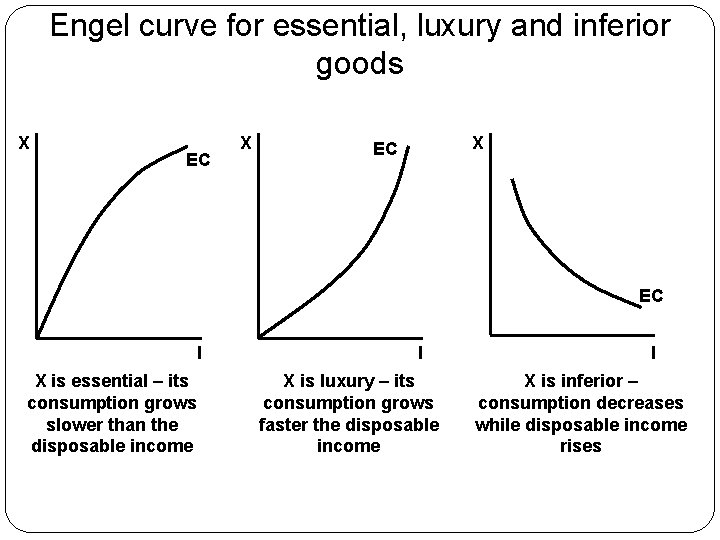
Engel Curve - EC Ø shows the relation between the volume of goods consumption and the disposable income

Engel curve - derivation Y ICC E 3 E 2 E 1 X I 2 I 1 X 2 X 3 I 3 X EC X 3 X 2 X 1 I 2 I 3 I

Engel curve for essential, luxury and inferior goods X EC X X EC EC I X is essential – its consumption grows slower than the disposable income I X is luxury – its consumption grows faster the disposable income I X is inferior – consumption decreases while disposable income rises

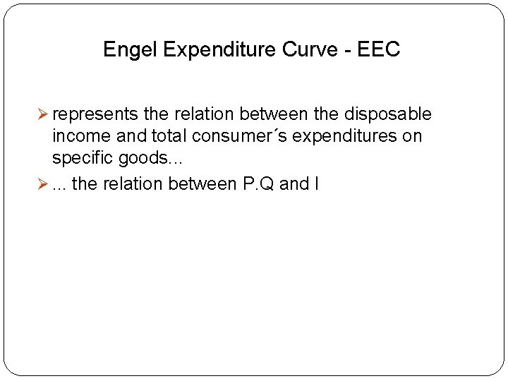
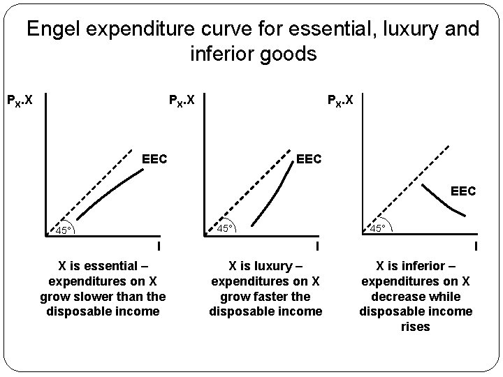
Engel Expenditure Curve - EEC Ø represents the relation between the disposable income and total consumer´s expenditures on specific goods. . . Ø. . . the relation between P. Q and I

Engel expenditure curve for essential, luxury and inferior goods PX. X EEC EEC 45° I X is essential – expenditures on X grow slower than the disposable income 45° I X is luxury – expenditures on X grow faster the disposable income I X is inferior – expenditures on X decrease while disposable income rises

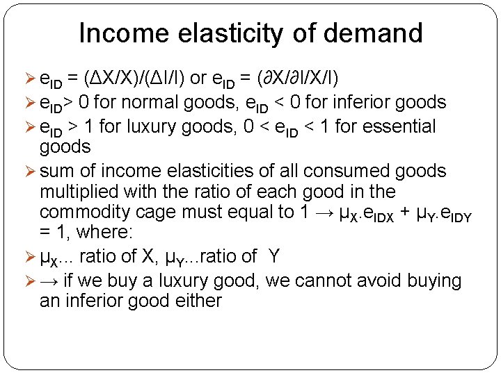
Income elasticity of demand Ø. . . reflects the sensitivity of consumer´s reaction to the change of disposable income and his/her consumption Ø it is a relative change of quantity demanded induced with the change of disposable income

Income elasticity of demand Ø e. ID = (ΔX/X)/(ΔI/I) or e. ID = (∂X/∂I/X/I) Ø e. ID> 0 for normal goods, e. ID < 0 for inferior goods Ø e. ID > 1 for luxury goods, 0 < e. ID < 1 for essential goods Ø sum of income elasticities of all consumed goods multiplied with the ratio of each good in the commodity cage must equal to 1 → μX. e. IDX + μY. e. IDY = 1, where: Ø μX. . . ratio of X, μY. . . ratio of Y Ø → if we buy a luxury good, we cannot avoid buying an inferior good either

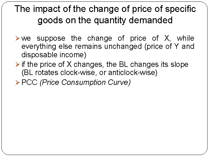
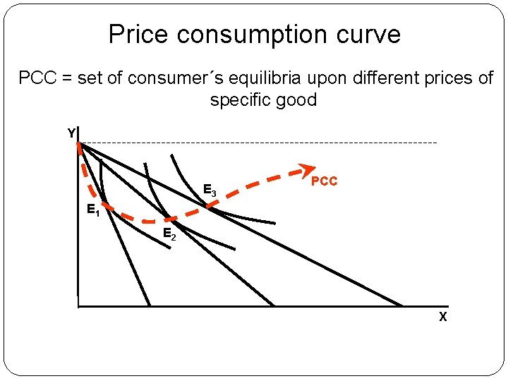
The impact of the change of price of specific goods on the quantity demanded Ø we suppose the change of price of X, while everything else remains unchanged (price of Y and disposable income) Ø if the price of X changes, the BL changes its slope (BL rotates clock-wise, or anticlock-wise) Ø PCC (Price Consumption Curve)

Price consumption curve PCC = set of consumer´s equilibria upon different prices of specific good Y E 3 PCC E 1 E 2 X

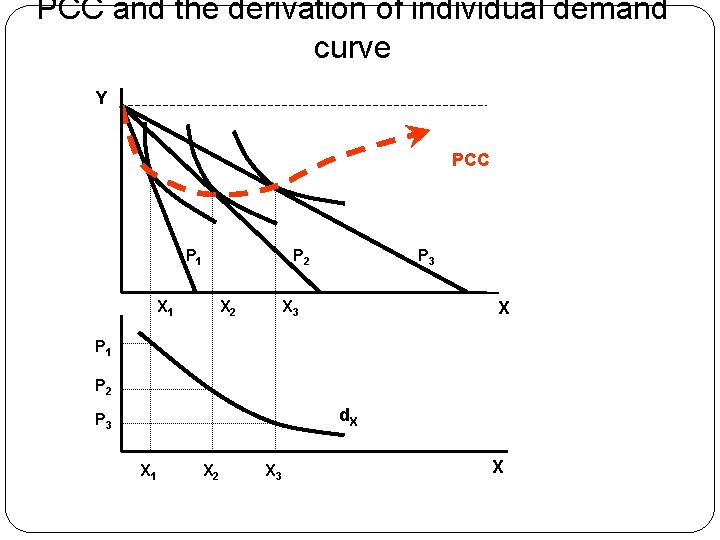
PCC and the derivation of individual demand curve Y PCC P 1 P 2 X 1 X 2 P 3 X P 1 P 2 d. X P 3 X 1 X 2 X 3 X

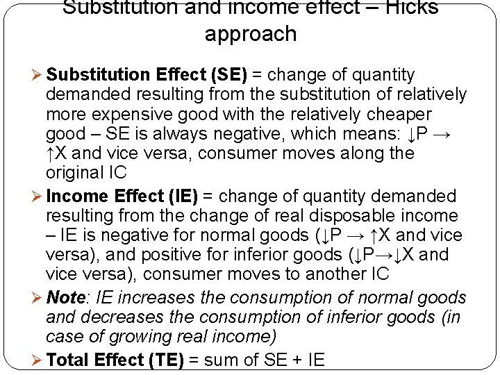
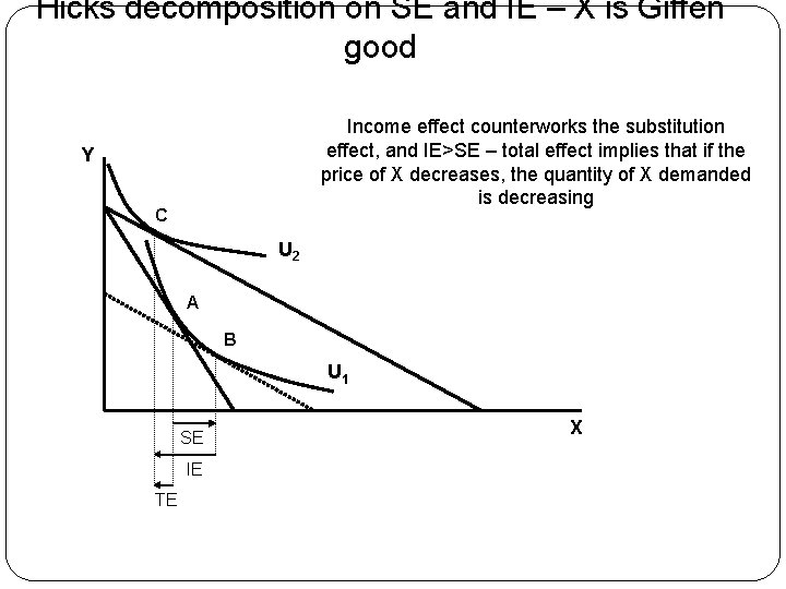
Substitution and income effect – Hicks approach Ø Substitution Effect (SE) = change of quantity demanded resulting from the substitution of relatively more expensive good with the relatively cheaper good – SE is always negative, which means: ↓P → ↑X and vice versa, consumer moves along the original IC Ø Income Effect (IE) = change of quantity demanded resulting from the change of real disposable income – IE is negative for normal goods (↓P → ↑X and vice versa), and positive for inferior goods (↓P→↓X and vice versa), consumer moves to another IC Ø Note: IE increases the consumption of normal goods and decreases the consumption of inferior goods (in case of growing real income) Ø Total Effect (TE) = sum of SE + IE

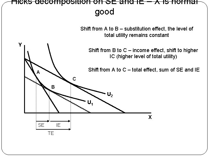
Hicks decomposition on SE and IE – X is normal good Shift from A to B – substitution effect, the level of total utility remains constant Y Shift from B to C – income effect, shift to higher IC (higher level of total utility) Shift from A to C – total effect, sum of SE and IE A C B U 2 U 1 X SE IE TE

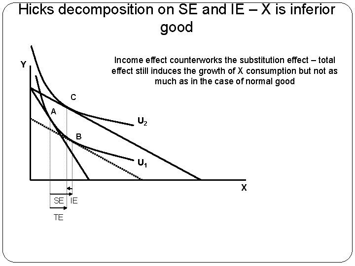
Hicks decomposition on SE and IE – X is inferior good Income effect counterworks the substitution effect – total effect still induces the growth of X consumption but not as much as in the case of normal good Y C A U 2 B U 1 X SE IE TE

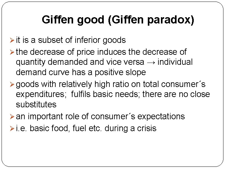
Giffen good (Giffen paradox) Ø it is a subset of inferior goods Ø the decrease of price induces the decrease of quantity demanded and vice versa → individual demand curve has a positive slope Ø goods with relatively high ratio on total consumer´s expenditures; fulfils basic needs; there are no close substitutes Ø an important role of consumer´s expectations Ø i. e. basic food, fuel etc. during a crisis

Hicks decomposition on SE and IE – X is Giffen good Income effect counterworks the substitution effect, and IE>SE – total effect implies that if the price of X decreases, the quantity of X demanded is decreasing Y C U 2 A B U 1 SE IE TE X

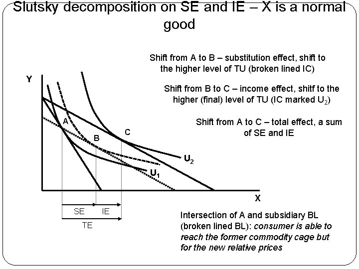
Slutsky approach to the SE and IE Ø different approach to the substitution effect resulting from the change of price of goods Ø Hicks SE – consumer is able to reach the constant level of total utility after the relative prices change Ø Slutsky SE – consumer is able to reach the former commodity cage after the change of relative prices Ø Slutsky´s SE includes some of the Hicks´s IE

Slutsky decomposition on SE and IE – X is a normal good Shift from A to B – substitution effect, shift to the higher level of TU (broken lined IC) Y Shift from B to C – income effect, shitf to the higher (final) level of TU (IC marked U 2) A Shift from A to C – total effect, a sum of SE and IE C B U 2 U 1 X SE TE IE Intersection of A and subsidiary BL (broken lined BL): consumer is able to reach the former commodity cage but for the new relative prices

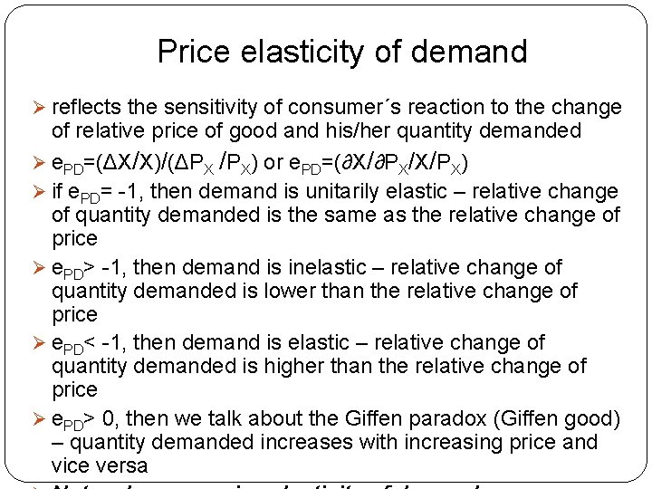
Price elasticity of demand Ø reflects the sensitivity of consumer´s reaction to the change of relative price of good and his/her quantity demanded Ø e. PD=(ΔX/X)/(ΔPX /PX) or e. PD=(∂X/∂PX/X/PX) Ø if e. PD= -1, then demand is unitarily elastic – relative change of quantity demanded is the same as the relative change of price Ø e. PD> -1, then demand is inelastic – relative change of quantity demanded is lower than the relative change of price Ø e. PD< -1, then demand is elastic – relative change of quantity demanded is higher than the relative change of price Ø e. PD> 0, then we talk about the Giffen paradox (Giffen good) – quantity demanded increases with increasing price and vice versa

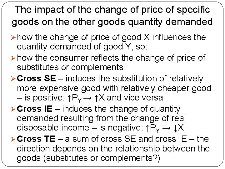
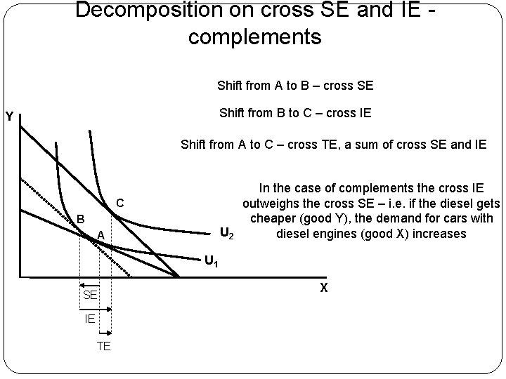
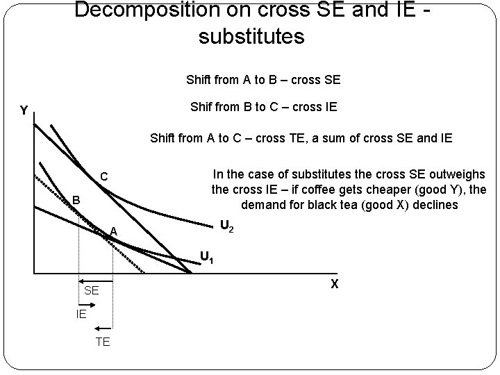
The impact of the change of price of specific goods on the other goods quantity demanded Ø how the change of price of good X influences the quantity demanded of good Y, so: Ø how the consumer reflects the change of price of substitutes or complements Ø Cross SE – induces the substitution of relatively more expensive good with relatively cheaper good – is positive: ↑PY → ↑X and vice versa Ø Cross IE – induces the change of quantity demanded resulting from the change of real disposable income – is negative: ↑PY → ↓X Ø Cross TE – a sum of cross SE and cross IE – the direction depends on the relationship between the goods (substitutes or complements? )

Decomposition on cross SE and IE complements Shift from A to B – cross SE Shift from B to C – cross IE Y Shift from A to C – cross TE, a sum of cross SE and IE C B U 2 A In the case of complements the cross IE outweighs the cross SE – i. e. if the diesel gets cheaper (good Y), the demand for cars with diesel engines (good X) increases U 1 SE IE TE X

Decomposition on cross SE and IE substitutes Shift from A to B – cross SE Shif from B to C – cross IE Y Shift from A to C – cross TE, a sum of cross SE and IE In the case of substitutes the cross SE outweighs the cross IE – if coffee gets cheaper (good Y), the demand for black tea (good X) declines C B U 2 A U 1 SE IE TE X

Task: What are the cross effects in the case of perfect complements and/or perfect substitutes?

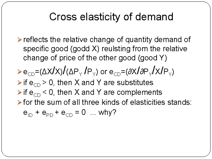
Cross elasticity of demand Ø reflects the relative change of quantity demand of specific good (godd X) reulsting from the relative change of price of the other good (good Y) / / Ø e. CD=(ΔX/X) (ΔPY /PY) or e. CD=(∂X/∂PY X/PY) Ø if e. CD > 0, then X and Y are substitutes Ø if e. CD < 0, then X and Y are complements Ø for the sum of all three kinds of elasticities stands: e. ID + e. PD + e. CD = 0. . . why?

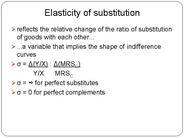
Elasticity of substitution Ø reflects the relative change of the ratio of substitution of goods with each other. . . Ø. . . a variable that implies the shape of indifference curves Ø σ = Δ(Y/X) : Δ(MRSC) Y/X MRSC Ø σ = ∞ for perfect substitutes Ø σ = 0 for perfect complements

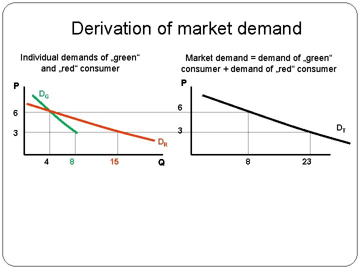
Derivation of market demand Ø market demand is the horizontal sum of all individual demands (demands of all consumers) for the specific good

Derivation of market demand Individual demands of „green“ and „red“ consumer P Market demand = demand of „green“ consumer + demand of „red“ consumer P DG 6 6 DT 3 3 DR 4 8 15 Q 8 23