2 2 NORMAL DISTRIBUTIONS HW P 131 41

2. 2 NORMAL DISTRIBUTIONS HW: P. 131 (41 -59 ODD, 63, 65, 66, 68 -74)

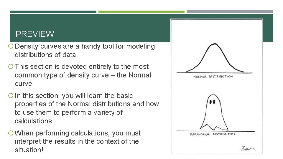
PREVIEW Density curves are a handy tool for modeling distributions of data. This section is devoted entirely to the most common type of density curve – the Normal curve. In this section, you will learn the basic properties of the Normal distributions and how to use them to perform a variety of calculations. When performing calculations, you must interpret the results in the context of the situation!

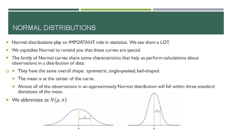
NORMAL DISTRIBUTIONS

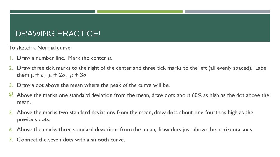
DRAWING PRACTICE!

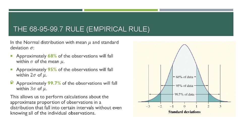
THE 68 -95 -99. 7 RULE (EMPIRICAL RULE)

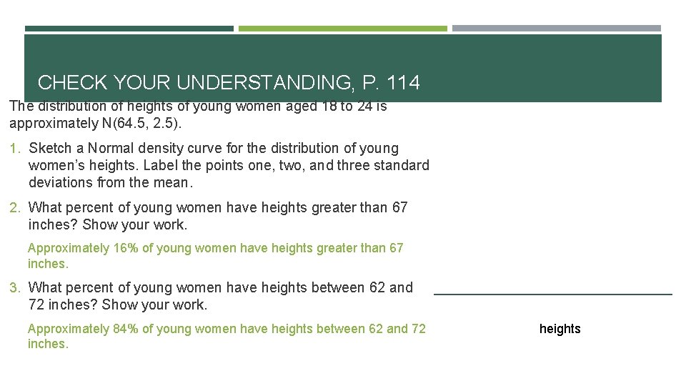
CHECK YOUR UNDERSTANDING, P. 114 The distribution of heights of young women aged 18 to 24 is approximately N(64. 5, 2. 5). 1. Sketch a Normal density curve for the distribution of young women’s heights. Label the points one, two, and three standard deviations from the mean. 2. What percent of young women have heights greater than 67 inches? Show your work. Approximately 16% of young women have heights greater than 67 inches. 3. What percent of young women have heights between 62 and 72 inches? Show your work. Approximately 84% of young women have heights between 62 and 72 inches. heights

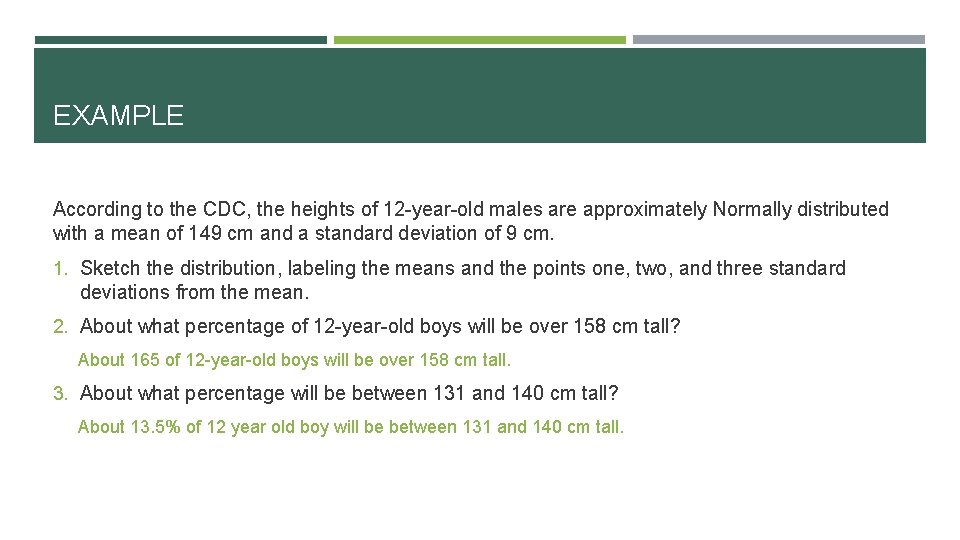
EXAMPLE According to the CDC, the heights of 12 -year-old males are approximately Normally distributed with a mean of 149 cm and a standard deviation of 9 cm. 1. Sketch the distribution, labeling the means and the points one, two, and three standard deviations from the mean. 2. About what percentage of 12 -year-old boys will be over 158 cm tall? About 165 of 12 -year-old boys will be over 158 cm tall. 3. About what percentage will be between 131 and 140 cm tall? About 13. 5% of 12 year old boy will be between 131 and 140 cm tall.

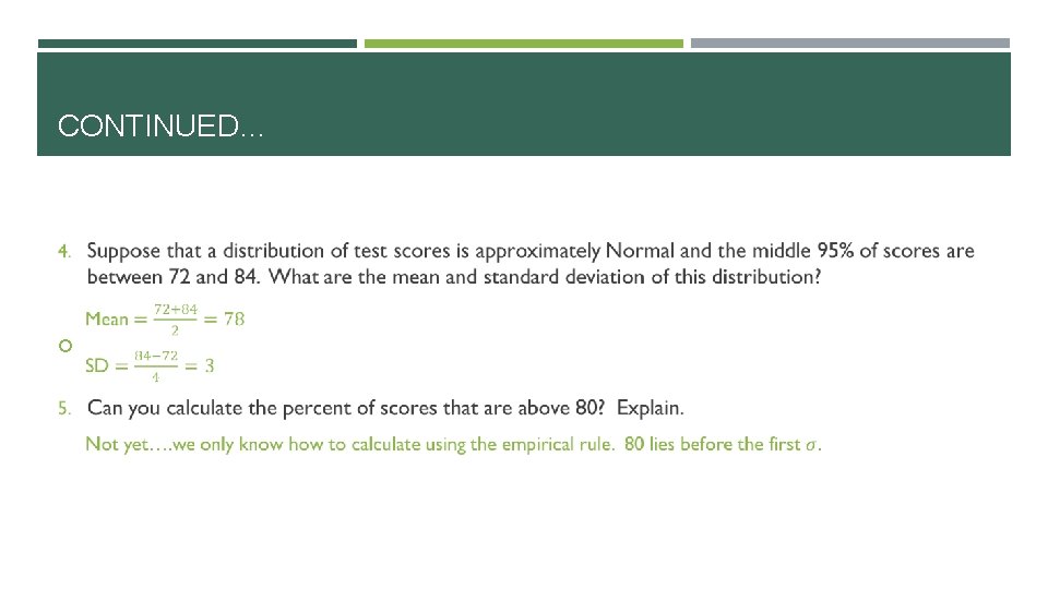
CONTINUED…

TIME TO PRACTICE!!! Complete the practice worksheet using the 68 -95 -99. 7 rule. Due tomorrow!!!

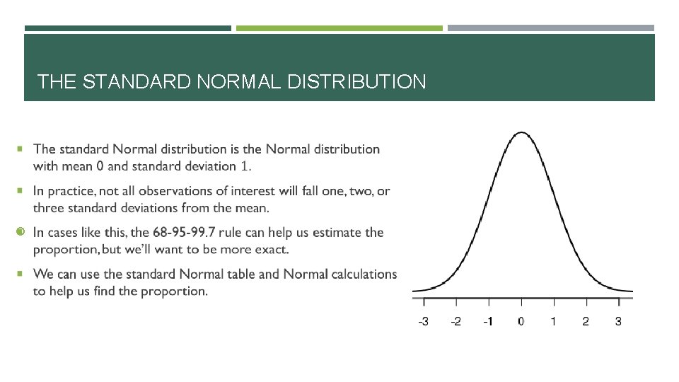
THE STANDARD NORMAL DISTRIBUTION

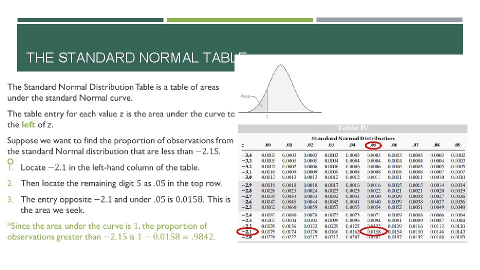
THE STANDARD NORMAL TABLE

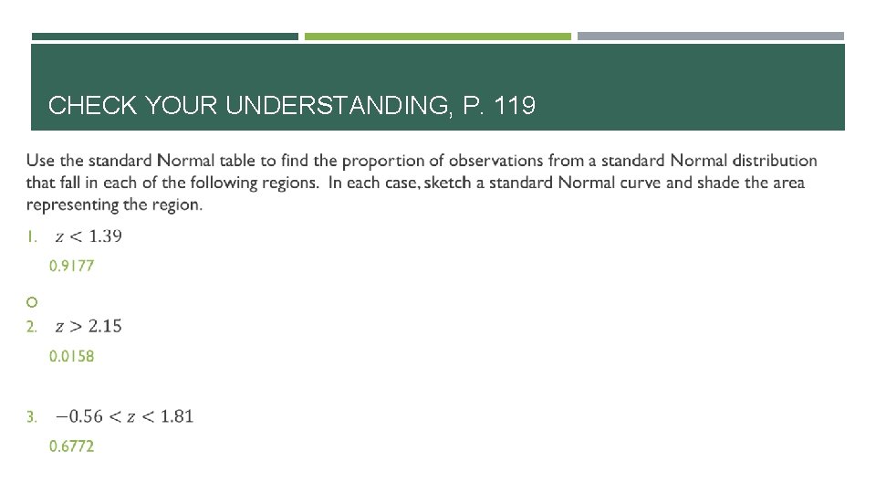
CHECK YOUR UNDERSTANDING, P. 119

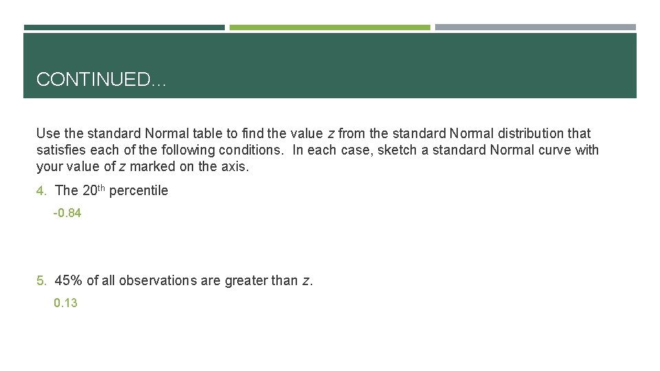
CONTINUED… Use the standard Normal table to find the value z from the standard Normal distribution that satisfies each of the following conditions. In each case, sketch a standard Normal curve with your value of z marked on the axis. 4. The 20 th percentile -0. 84 5. 45% of all observations are greater than z. 0. 13

NORMAL DISTRIBUTION CALCULATIONS We can answer a question about proportions of any Normal distribution by standardizing and then using the standard Normal table. Follow the four-step process: 1. STATE: Express the problem in terms of a variable x. 2. PLAN: Sketch a picture of the distribution and shade the area of interest. 3. DO: Perform calculations by standardizing x and then using Table A or your calculator to find the required area under the Normal curve. 4. CONCLUDE: Write your conclusion in the context of the problem.

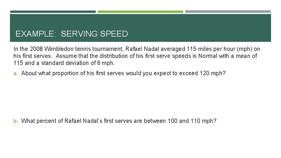
EXAMPLE: SERVING SPEED In the 2008 Wimbledon tennis tournament, Rafael Nadal averaged 115 miles per hour (mph) on his first serves. Assume that the distribution of his first serve speeds is Normal with a mean of 115 and a standard deviation of 6 mph. a. About what proportion of his first serves would you expect to exceed 120 mph? b. What percent of Rafael Nadal’s first serves are between 100 and 110 mph?

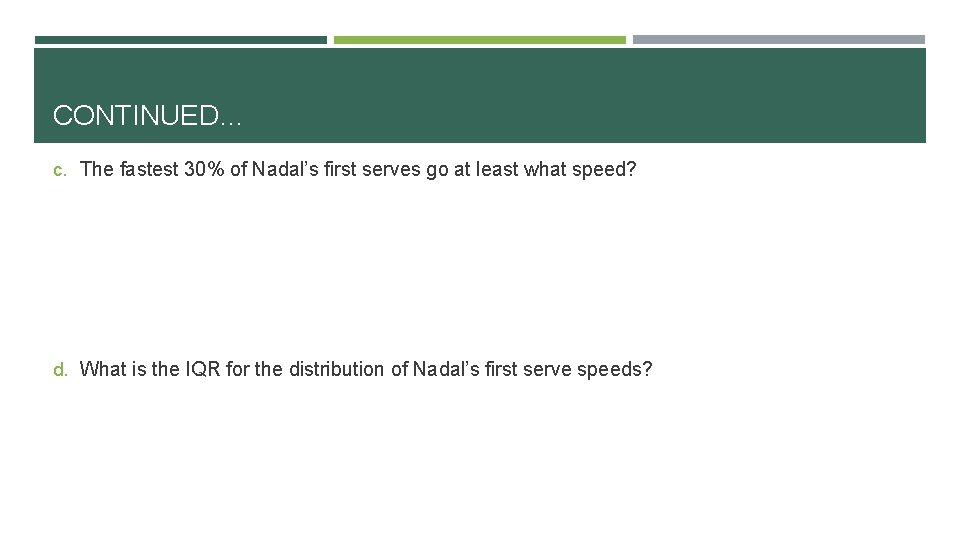
CONTINUED… c. The fastest 30% of Nadal’s first serves go at least what speed? d. What is the IQR for the distribution of Nadal’s first serve speeds?

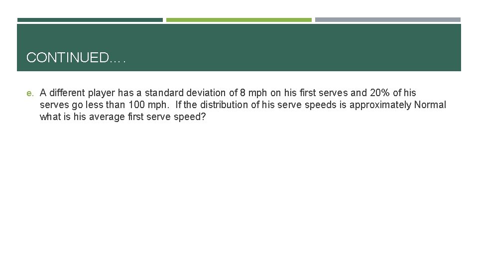
CONTINUED…. e. A different player has a standard deviation of 8 mph on his first serves and 20% of his serves go less than 100 mph. If the distribution of his serve speeds is approximately Normal what is his average first serve speed?

TIME TO PRACTICE! Complete the practice worksheet using the standard Normal table. Due tomorrow!!!

YIPPEE!!! Your calculator will do Normal calculations for you!!!

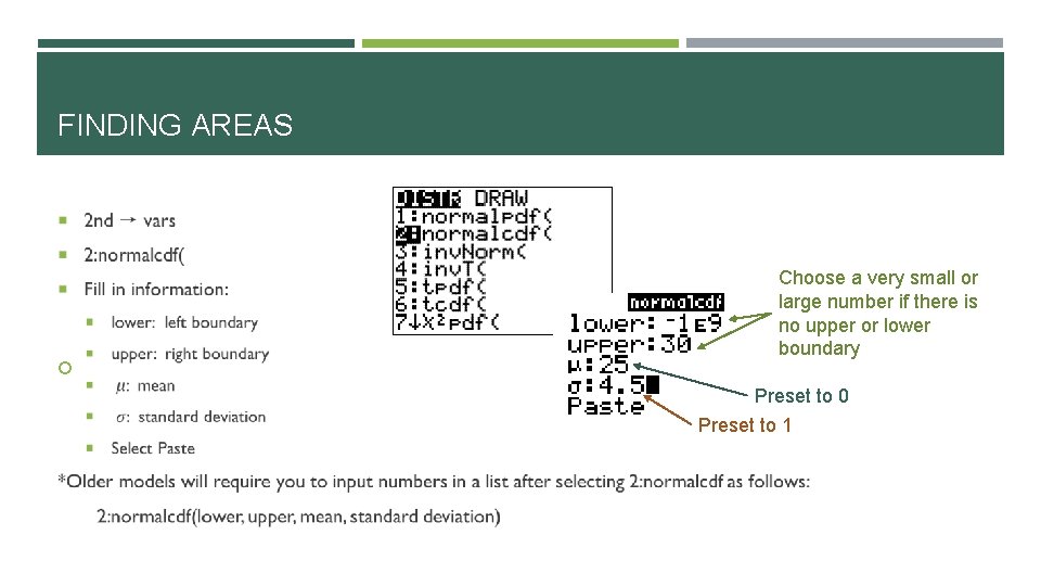
FINDING AREAS Choose a very small or large number if there is no upper or lower boundary Preset to 0 Preset to 1

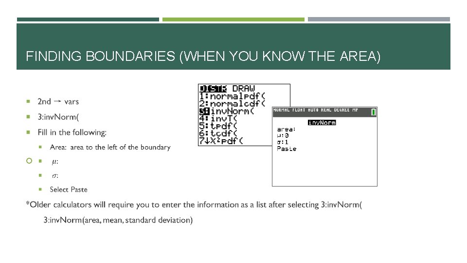
FINDING BOUNDARIES (WHEN YOU KNOW THE AREA)

AP TIP When you show work on the AP Exam, you will lose credit for “calculator speak. ” You must show your work on Normal calculation questions or specify the operation and values you are using in your calculator!

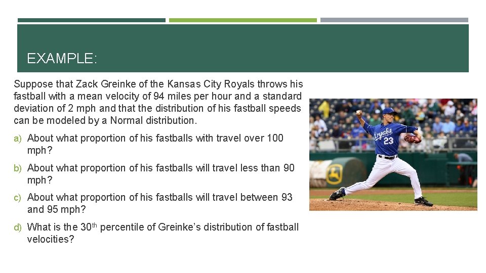
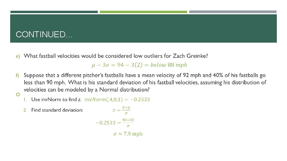
EXAMPLE: Suppose that Zack Greinke of the Kansas City Royals throws his fastball with a mean velocity of 94 miles per hour and a standard deviation of 2 mph and that the distribution of his fastball speeds can be modeled by a Normal distribution. a) About what proportion of his fastballs with travel over 100 mph? b) About what proportion of his fastballs will travel less than 90 mph? c) About what proportion of his fastballs will travel between 93 and 95 mph? d) What is the 30 th percentile of Greinke’s distribution of fastball velocities?

CONTINUED…

ASSESSING NORMALITY Just because a distribution is symmetric, single-peaked, and bell-shaped, it is NOT necessarily Normal. Before performing Normal calculations, you should be sure the distribution you are exploring really is Normal. There are two methods to check for Normality: 68 -95 -99. 7 rule Probability Plots

68 -95 -99. 7 RULE FOR ASSESSING NORMALITY 1. Plot the data. Make a dotplot, stemplot, or histogram. See if the graph is approximately symmetric and bell-shaped. 2. Check whether the data follow the 68 -95 -99. 7 rule. Count the number of observations within one, two, and three standard deviations of the mean.

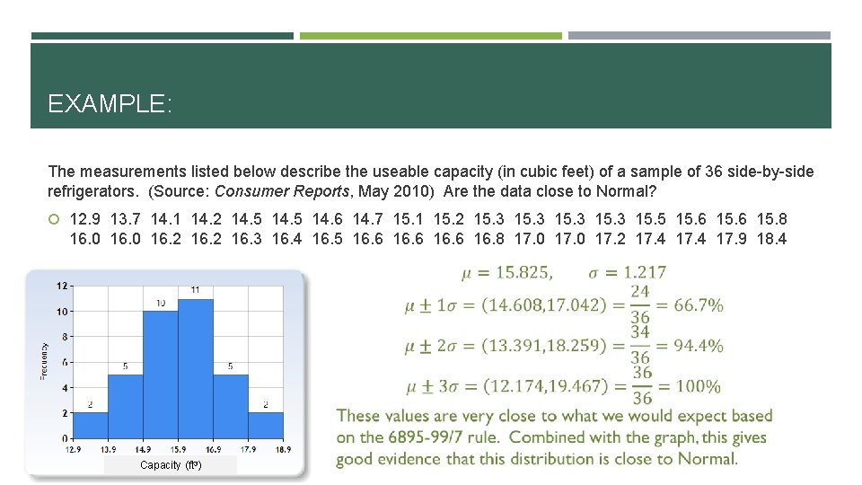
EXAMPLE: The measurements listed below describe the useable capacity (in cubic feet) of a sample of 36 side-by-side refrigerators. (Source: Consumer Reports, May 2010) Are the data close to Normal? 12. 9 13. 7 14. 1 14. 2 14. 5 14. 6 14. 7 15. 1 15. 2 15. 3 15. 5 15. 6 15. 8 16. 0 16. 2 16. 3 16. 4 16. 5 16. 6 16. 8 17. 0 17. 2 17. 4 17. 9 18. 4 Capacity (ft 3)

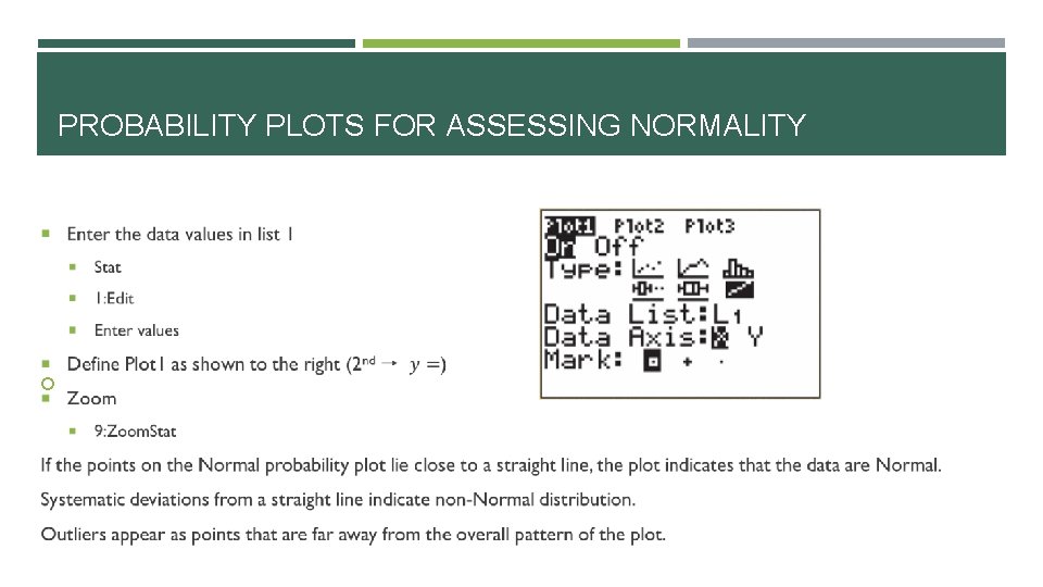
PROBABILITY PLOTS FOR ASSESSING NORMALITY

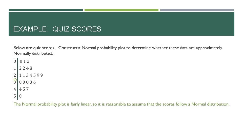
EXAMPLE: QUIZ SCORES