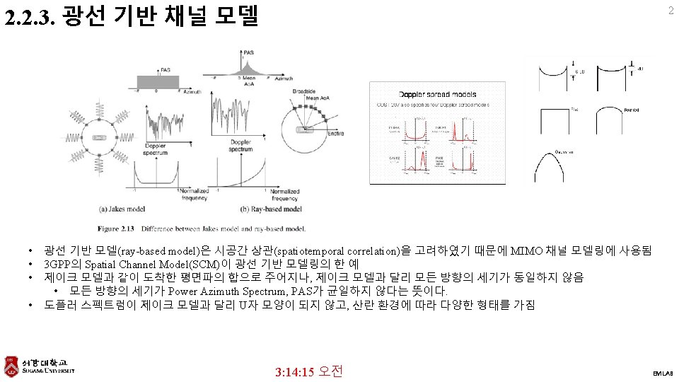
2 2 4 Power Delay Profile PDP PDP

2. 2. 4. 주파수 선택적 페이딩 채널 모델 • • 주파수 선택적 페이딩 채널을 모델링하기 위해 전력 지연 프로파일(Power Delay Profile, PDP)가 필요함 PDP는 각 경로의 평균 전력과 지연을 나타냄 보행자 A 보행자 B 차량 A 차량 B 도플러 상대 지연 평균 전력 스펙트럼 [ns] [d. B] 1 0 0 -2. 5 Classic 탭 2 110 -9. 7 200 -0. 9 310 -1. 0 300 0. 0 Classic 3 190 -19. 2 800 -4. 9 710 -9. 0 8900 -12. 8 Classic 4 410 -22. 8 1200 -8. 0 1090 -10. 0 12900 -10. 0 Classic 5 2300 -7. 8 1730 -15. 0 17100 -25. 2 Classic 6 3700 -23. 9 2510 -20. 0 20000 -16. 0 Classic ITU-R 모델의 PDP 탭 1 2 3 4 5 6 8 Typical urban (TU) Bad urban (BU) Typical rural area (RA) 상대 지연 평균 전력 도플러 [us] 스펙트럼 0. 0 0. 189 Classic 0. 0 0. 164 Classic 0. 0 0. 602 RICE 0. 2 0. 379 Classic 0. 3 0. 293 Classic 0. 1 0. 241 Classic 0. 5 0. 239 Classic 1. 0 0. 147 GAUS 1 0. 2 0. 096 Classic 1. 6 0. 095 GAUS 1 1. 6 0. 094 GAUS 1 0. 3 0. 036 Classic 2. 3 0. 061 GAUS 2 5. 0 0. 185 GAUS 2 0. 4 0. 018 Classic 5. 0 0. 037 GAUS 2 6, 6 0. 117 GAUS 2 0. 5 0. 006 Classic 탭 1 2 3 4 5 6 7 8 9 10 11 12 Typical urban (TU) Bad urban (BU) 상대 지연 평균 전력 도플러 [us] 스펙트럼 0. 092 Classic 0. 033 Classic 0. 115 Classic 0. 1 0. 089 Classic 0. 3 0. 231 Classic 0. 3 0. 141 Classic 0. 5 0. 127 Classic 0. 7 0. 194 GAUS 1 0. 8 0. 115 GAUS 1 1. 6 0. 114 GAUS 1 1. 1 0. 074 GAUS 1 2. 2 0. 052 GAUS 2 1. 3 0. 046 GAUS 1 3. 1 0. 035 GAUS 2 1. 7 0. 074 GAUS 1 5. 0 0. 140 GAUS 2 2. 3 0. 051 GAUS 2 6. 0 0. 136 GAUS 2 3. 1 0. 032 GAUS 2 7. 2 0. 041 GAUS 2 3. 2 0. 018 GAUS 2 8. 1 0. 019 GAUS 2 5. 0 0. 025 GAUS 2 10. 006 GAUS 2 COST 207 모델의 PDP 3: 14: 20 오전 EMLAB

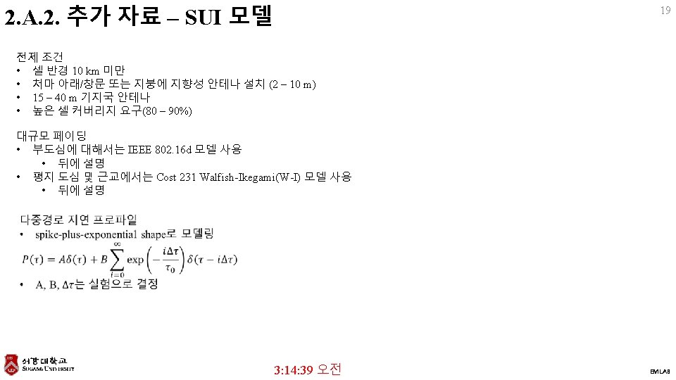
2. 2. 5. SUI 채널 모델 – 파라미터 SUI 1 SUI 2 SUI 3 12 SUI 4 SUI 5 SUI 6 Imp Tap number 1 2 3 1 2 3 Delay [us] 0 0. 4 0. 9 0 0. 4 1. 1 0 0. 4 0. 9 0 1. 5 4 0 4 10 0 14 20 Power (omni ant. ) [d. B] 0 -15 -20 0 -12 -15 0 -5 -10 0 -4 -8 0 -5 -10 0 -14 Powers 90% K-factor (omni) 4 0 0 2 0 0 1 0 0 0 75% K-factor (omni) 20 0 0 11 0 0 7 0 0 1 0 0 0 0 50% K-factor (omni) - - - 2 0 0 1 0 0 Power (30° ant. ) [d. B] 0 -21 -32 0 -18 -27 0 -11 -22 0 -10 -20 0 -11 -22 0 -16 -26 90% K-factor(30° ant. ) 16 0 0 8 0 0 3 0 0 1 0 0 0 0 75% K-factor (30° ant. ) 72 0 0 36 0 0 19 0 0 5 0 0 2 0 0 50% K-factor (30° ant. ) - - - 7 0 0 5 0 0 Doppler [Hz] 0. 4 Terrain type (802. 16 d 참조) 0. 3 SUI 1 0. 5 0. 2 0. 15 0. 3 0. 5 SUI 20. 25 0. 4 SUI 3 0. 2 0. 15 0. 25 SUI 5 2 1. 5 SUI 4 2. 5 SUI 6 0. 4 0. 3 0. 7 0. 5 0. 4 0. 3 0. 5 0. 3 0 2 3 4 4 4 -0. 1771 -0. 3930 -1. 5113 -1. 9218 -1. 5113 -0. 5683 -0. 0371 -0. 0768 -0. 3573 -0. 4532 -0. 3573 -0. 1184 C C B B A A 3: 14: 28 오전 Delays Ks 0. 5 Imp. Dopplers Ant_corrs Fnorms EMLAB

2. 2. 5. SUI 채널 모델 – 파라미터 SUI 1 SUI 2 13 SUI 4 SUI 5 SUI 6 0. 111 0. 202 0. 264 1. 257 2. 842 5. 240 overall K 90% 3. 3 16 0. 5 0. 2 0. 1 75% 10. 4 5. 1 1. 6 0. 3 50% - - 1. 0 0. 042 0. 69 0. 123 0. 563 1. 276 2. 370 overall K 90% 14. 0 6. 9 2. 2 1. 0 0. 4 75% 44. 2 21. 8 7. 0 3. 2 1. 3 50% - - 4. 2 SUI_parameters가 조건 입력에 따라 파라미터 선택해주는 프로그램 • Omni 안테나, K-factor 90%에 대해서만 구현 • 지연 확산에 대해서는 파라미터 출력이 없음 3: 14: 32 오전 EMLAB

2. 2. 5. SUI 채널 모델 – 프로그램 14 function [Fad. Mtx, tf]=SUI_fading(P_d. B, K_factor, Dopplershift_Hz, Fnorm_d. B, N, M, Nfosf) % SUI fading generation using FWGN with fitering in the frequency domain % Inputs: % P_d. B : power in each tap in d. B % K_factor : Rician K-factor in linear scale % Dopplershift_Hz : a vector containing the maximum Doppler frequency of each path in Hz % Fnorm_d. B : gain normalization factor in d. B % N : # of independent random realization % M : length of Doppler filter, i. e, size of IFFT % Nfosf : fading oversampling factor % Outputs: % Fad. Mtx : length(P_d. B) x N fading matrix % tf : fading sample time=1/(Max. Doppler BW * Nfosf) Power = 10. ^(P_d. B/10); % calculate linear power s 2 = Power. /(K_factor+1); % calculate variance s=sqrt(s 2); m 2 = Power. *(K_factor. /(K_factor+1)); % calculate constant power m = sqrt(m 2); % calculate constant part L=length(Power); % # of tabs fmax= max(Dopplershift_Hz); tf=1/(2*fmax*Nfosf); if isscalar(Dopplershift_Hz), Dopplershift_Hz= Dopplershift_Hz*ones(1, L); path_wgn= sqrt(1/2)*complex(randn(L, N), randn(L, N)); for p=1: L filt=gen_filter(Dopplershift_Hz(p), fmax, M, Nfosf, 'sui'); path(p, : )=fftfilt(filt, [path_wgn(p, : ) zeros(1, M)]); %filtering WGN end Fad. Mtx= path(: , M/2+1: end-M/2); for i=1: L , Fad. Mtx(i, : )=Fad. Mtx(i, : )*s(i) + m(i)*ones(1, N); end Fad. Mtx = Fad. Mtx*10^(Fnorm_d. B/20); 3: 14: 34 오전 end EMLAB

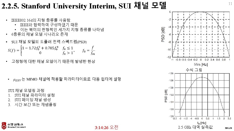
2. 2. 5. SUI 채널 모델 – 결과 15 초기화 clear, clf • workspace 초기화 ch_no=6; fc=2 e 9; • 피규어창 닫기 fs_Hz=1 e 7; 설정 Nfading=1024; % Size of Doppler filter • SUI 시나리오 6 N=10000; • 주파수 2 GHz Nos=4; • fs 10 MHz [Delay_us, P_d. B, K_factor, Dopplershift_Hz, Ant_corr, Fnorm_d. B]=SUI_parameters(ch_no); [Fad. Time, tf]=SUI_fading(P_d. B, K_factor, Dopplershift_Hz, Fnorm_d. B, N, Nfading, Nos); • 도플러 필터 탭 수 1024 K 1= size(Fad. Time, 2)-1; • 도플러 주파수 오버샘플링 배율 4 c_table=['b'; 'r'; 'k'; 'm']; subplot(311) stem(Delay_us, 10. ^(P_d. B/10)); PDP 선형값 출력 grid on, xlabel('Delay time[ms]'), ylabel('Channel gain'); title(['PDP of Channel No. ', num 2 str(ch_no)]), set(gca, 'fontsize', 9) subplot(312) for k=1: length(P_d. B) plot([0: K 1]*tf, 20*log 10(abs(Fad. Time(k, : ))), c_table(k, : )); hold on end grid on, xlabel('Time[s]'), ylabel('Channel Power[d. B]'); title(['Channel No. ', num 2 str(ch_no)]), axis([0 60 -50 10]) legend('Path 1', 'Path 2', 'Path 3'), set(gca, 'fontsize', 9) idx_nonz= find(Dopplershift_Hz); Fad. Freq= ones(length(Dopplershift_Hz), Nfading); for k=1: length(idx_nonz) max_dsp= 2*Nos*max(Dopplershift_Hz); dfmax= max_dsp/Nfading; % Doppler frequency spacing respect to maximal Doppler frequency Nd= floor(Dopplershift_Hz(k)/dfmax)-1; f 0 = [-Nd+1: Nd]/Nd; % frequency vector f = f 0. *Dopplershift_Hz(k); tmp=0. 785*f 0. ^4 - 1. 72*f 0. ^2 + 1. 0; hpsd=psd(spectrum. welch, Fad. Time(idx_nonz(k), : ), 'Fs', max_dsp, 'Spectrum. Type', 'twosided'); nrom_f=hpsd. Frequencies-mean(hpsd. Frequencies); PSD_d=fftshift(hpsd. Data); subplot(3, 3, 6+k), plot(nrom_f, PSD_d, 'b', f, tmp, 'r') 각 탭의 도플러 스펙트럼 계산값(PSD_d)과 이론적인 PSD(tmp) 출력 xlabel('Frequency[Hz]'), axis([-1 1 0 1. 1*max([PSD_d. ' tmp])]) title(['h_', num 2 str(idx_nonz(k)), ' path']); set(gca, 'fontsize', 9) end 3: 14: 35 오전 EMLAB

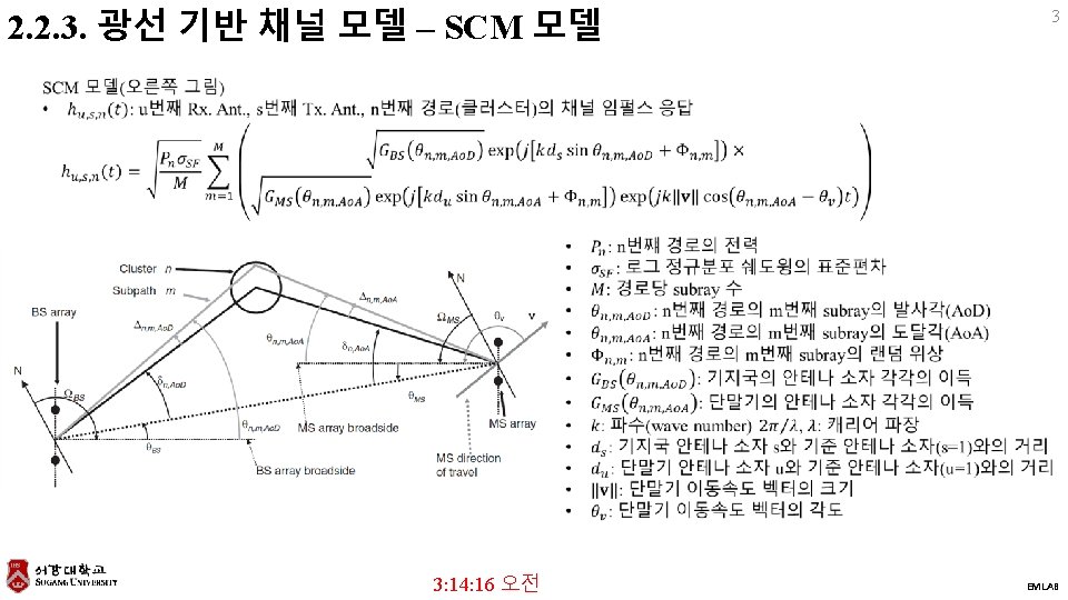
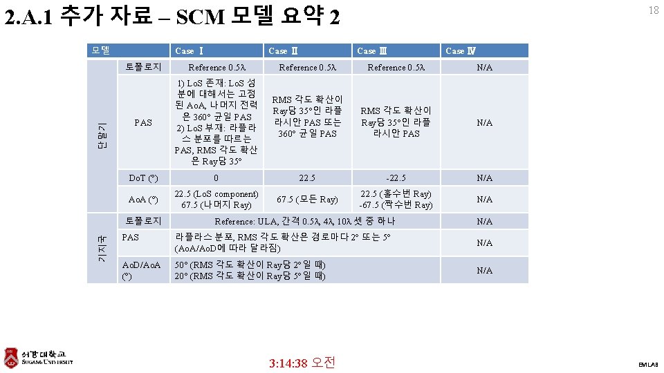
2. A. 1 추가 자료 – SCM 모델 요약 1 모델 Case Ⅰ 17 Case Ⅱ Case Ⅲ Case Ⅳ Case C Case D Case A 3 GPP 2 제안 기존 모델 Model A, D, E Model C Model B Model F PDP 수정된 보행자 A 차량 A 보행자 B 단일경로 경로 수 1) 4+1 (Lo. S 존재, K=6 d. B) 2) 4 (Lo. S 없음) 6 6 1 지연 (ns) Case B 상대 경로 전력 (d. B) 3 GPP 제안 기존 모델 속도 (kph) 1) 0. 0 2) –inf 0 0 1) -6. 51 2) 0. 0 0 -1. 0 310 -0. 9 200 1) -16. 21 2) -9. 7 110 -9. 0 710 -4. 9 800 1) -25. 71 2) -19. 2 190 -10. 0 1090 -8. 0 1200 1) -29. 31 2) -22. 8 410 -15. 0 1730 -7. 8 2300 -20. 0 2510 -23. 9 3700 1) 3 2) 30, 120 3, 30, 120 3: 14: 38 오전 3, 30, 120 0 0 3 EMLAB

2. A. 2. 2 Cost 231 Walfish-Ikegami (W-I) 모델 3: 14: 41 오전 22 EMLAB

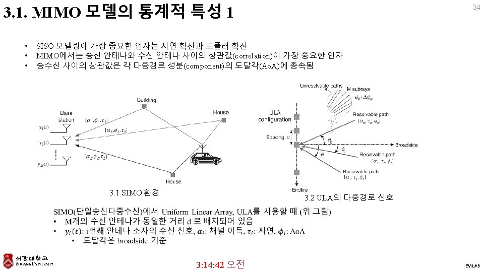
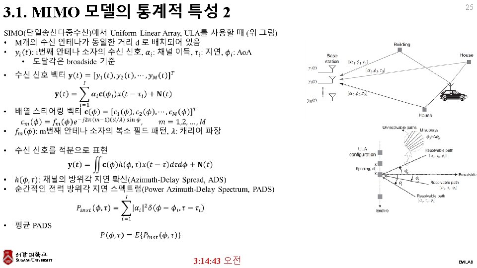
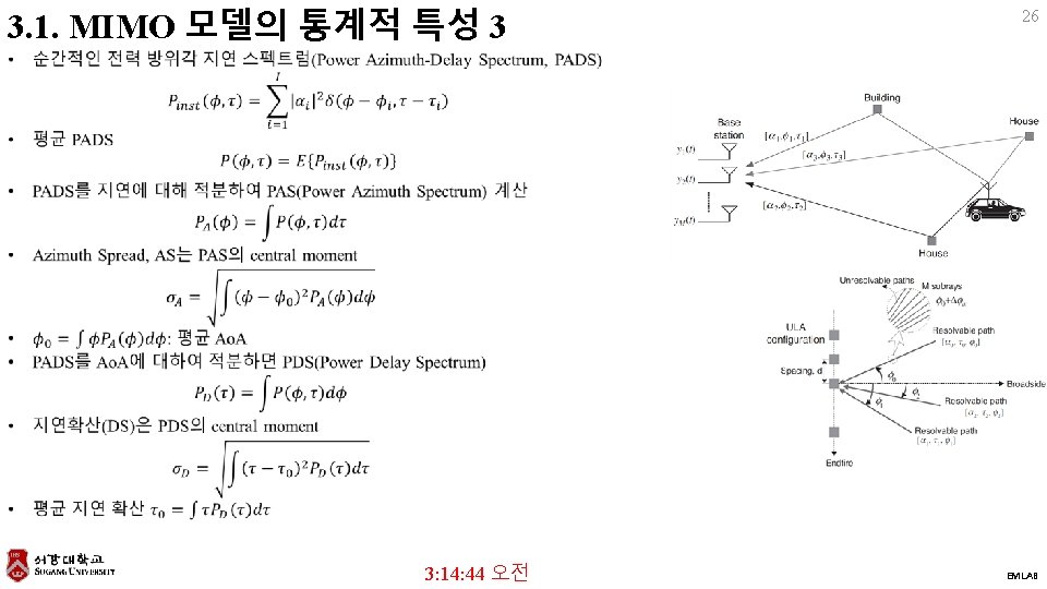
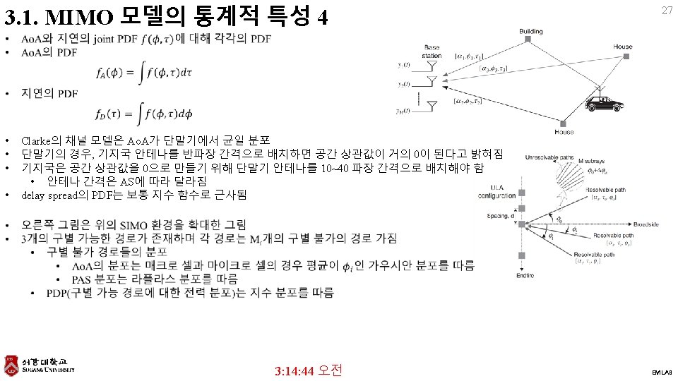
23 MATLAB을 사용한 MIMO OFDM 무선 통신 3. MIMO 채널 모델 3. 1 MIMO 모델의 통계 특성(Statistical MIMO Model) 3: 14: 42 오전 EMLAB

28 3. 1. 1. spatial correlation 1 3: 14: 45 오전 EMLAB

29 3. 1. 1. spatial correlation 2 3: 14: 46 오전 EMLAB

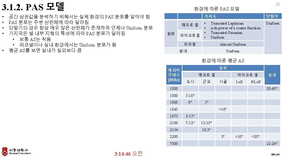
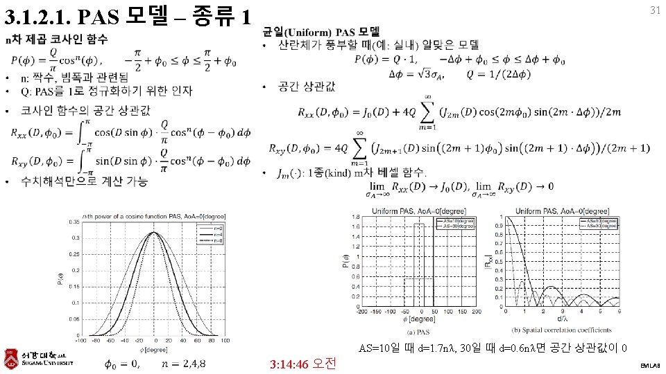
3. 1. 2. 1. PAS 모델 – 종류 2 32 3: 14: 47 오전 EMLAB

3. 1. 2. 1. PAS 모델 – 종류 3 33 3: 14: 48 오전 EMLAB