2 1 Supply and Demand The Supply Curve

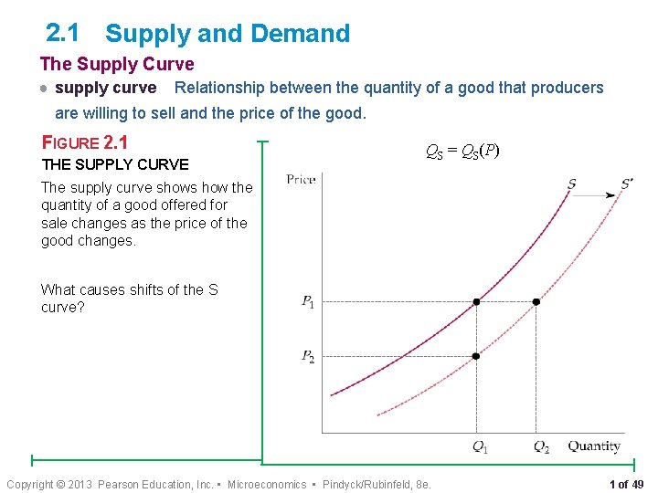
2. 1 Supply and Demand The Supply Curve ● supply curve Relationship between the quantity of a good that producers are willing to sell and the price of the good. FIGURE 2. 1 THE SUPPLY CURVE QS = QS(P) The supply curve shows how the quantity of a good offered for sale changes as the price of the good changes. What causes shifts of the S curve? Copyright © 2013 Pearson Education, Inc. • Microeconomics • Pindyck/Rubinfeld, 8 e. 1 of 49

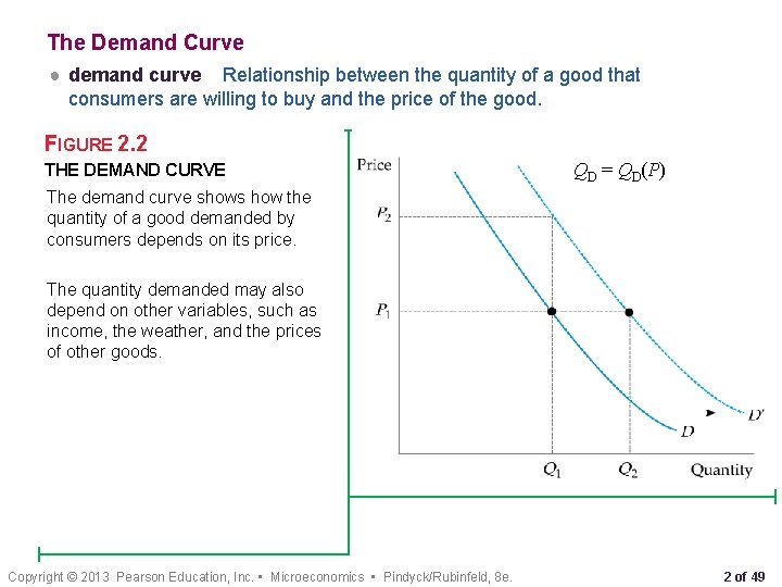
The Demand Curve ● demand curve Relationship between the quantity of a good that consumers are willing to buy and the price of the good. FIGURE 2. 2 THE DEMAND CURVE QD = QD(P) The demand curve shows how the quantity of a good demanded by consumers depends on its price. The quantity demanded may also depend on other variables, such as income, the weather, and the prices of other goods. Copyright © 2013 Pearson Education, Inc. • Microeconomics • Pindyck/Rubinfeld, 8 e. 2 of 49

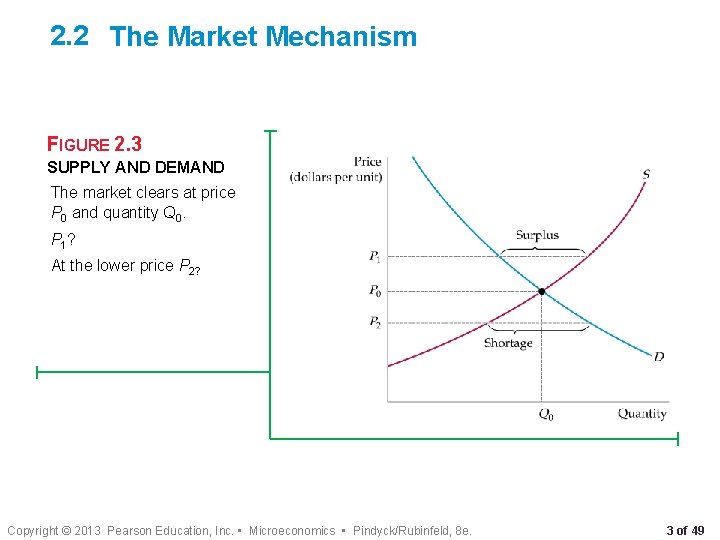
2. 2 The Market Mechanism FIGURE 2. 3 SUPPLY AND DEMAND The market clears at price P 0 and quantity Q 0. P 1? At the lower price P 2? Copyright © 2013 Pearson Education, Inc. • Microeconomics • Pindyck/Rubinfeld, 8 e. 3 of 49

WHEN CAN WE USE THE SUPPLY-DEMAND MODEL? We are assuming that at any given price, a given quantity will be produced and sold. This assumption makes sense only if a market is at least roughly competitive. By this we mean that both sellers and buyers should have little market power— i. e. , little ability individually to affect the market price. Suppose instead that supply were controlled by a single producer—a monopolist. If the demand curve shifts in a particular way, it may be in the monopolist’s interest to keep the quantity fixed but change the price, or to keep the price fixed and change the quantity. Copyright © 2013 Pearson Education, Inc. • Microeconomics • Pindyck/Rubinfeld, 8 e. 4 of 49

2. 3 Changes in Market Equilibrium What happens to equilibrium when supply and/or demand shift? Copyright © 2013 Pearson Education, Inc. • Microeconomics • Pindyck/Rubinfeld, 8 e. 5 of 49

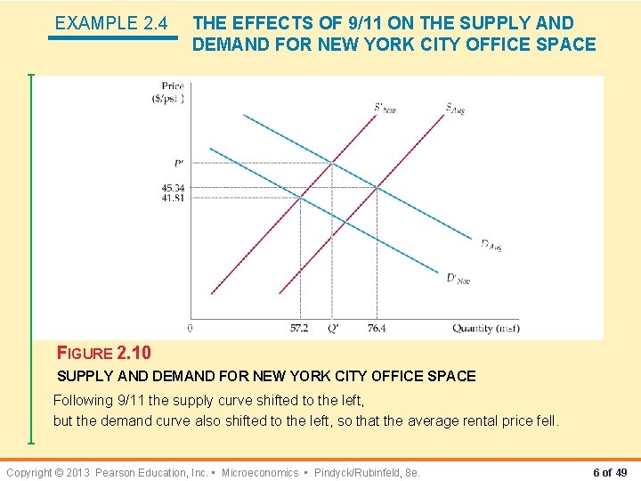
EXAMPLE 2. 4 THE EFFECTS OF 9/11 ON THE SUPPLY AND DEMAND FOR NEW YORK CITY OFFICE SPACE FIGURE 2. 10 SUPPLY AND DEMAND FOR NEW YORK CITY OFFICE SPACE Following 9/11 the supply curve shifted to the left, but the demand curve also shifted to the left, so that the average rental price fell. Copyright © 2013 Pearson Education, Inc. • Microeconomics • Pindyck/Rubinfeld, 8 e. 6 of 49

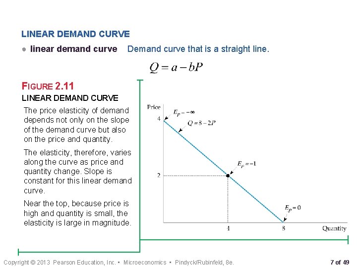
LINEAR DEMAND CURVE ● linear demand curve Demand curve that is a straight line. FIGURE 2. 11 LINEAR DEMAND CURVE The price elasticity of demand depends not only on the slope of the demand curve but also on the price and quantity. The elasticity, therefore, varies along the curve as price and quantity change. Slope is constant for this linear demand curve. Near the top, because price is high and quantity is small, the elasticity is large in magnitude. Copyright © 2013 Pearson Education, Inc. • Microeconomics • Pindyck/Rubinfeld, 8 e. 7 of 49

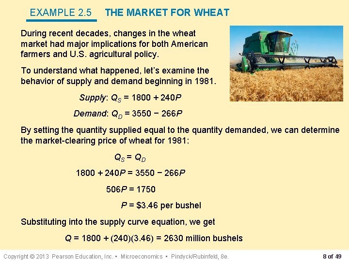
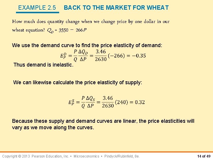
EXAMPLE 2. 5 THE MARKET FOR WHEAT During recent decades, changes in the wheat market had major implications for both American farmers and U. S. agricultural policy. To understand what happened, let’s examine the behavior of supply and demand beginning in 1981. Supply: QS = 1800 + 240 P Demand: QD = 3550 − 266 P By setting the quantity supplied equal to the quantity demanded, we can determine the market-clearing price of wheat for 1981: QS = QD 1800 + 240 P = 3550 − 266 P 506 P = 1750 P = $3. 46 per bushel Substituting into the supply curve equation, we get Q = 1800 + (240)(3. 46) = 2630 million bushels Copyright © 2013 Pearson Education, Inc. • Microeconomics • Pindyck/Rubinfeld, 8 e. 8 of 49

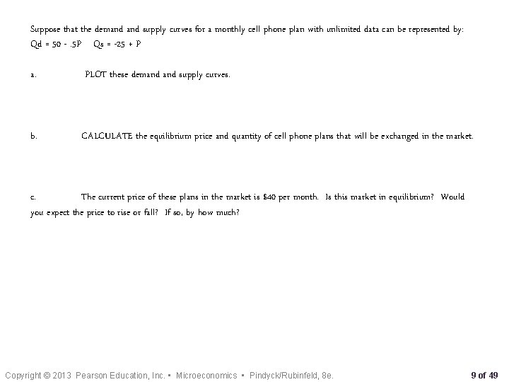
Suppose that the demand supply curves for a monthly cell phone plan with unlimited data can be represented by: Qd = 50 -. 5 P Qs = -25 + P a. PLOT these demand supply curves. b. CALCULATE the equilibrium price and quantity of cell phone plans that will be exchanged in the market. c. The current price of these plans in the market is $40 per month. Is this market in equilibrium? Would you expect the price to rise or fall? If so, by how much? Copyright © 2013 Pearson Education, Inc. • Microeconomics • Pindyck/Rubinfeld, 8 e. 9 of 49

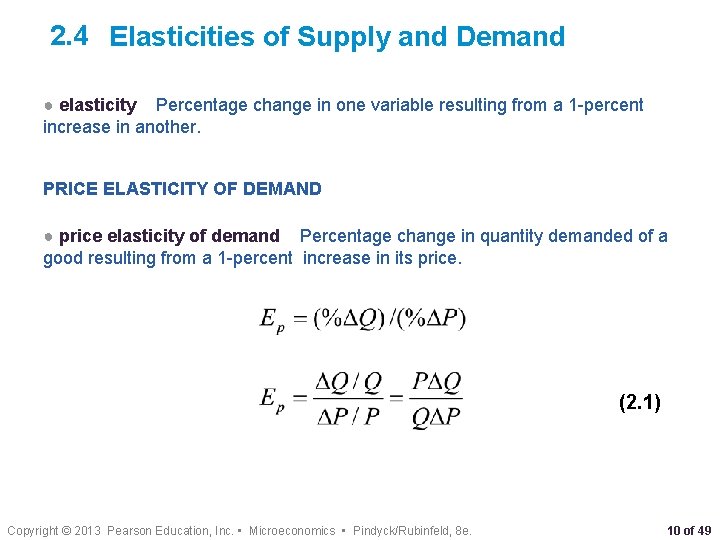
2. 4 Elasticities of Supply and Demand ● elasticity Percentage change in one variable resulting from a 1 -percent increase in another. PRICE ELASTICITY OF DEMAND ● price elasticity of demand Percentage change in quantity demanded of a good resulting from a 1 -percent increase in its price. (2. 1) Copyright © 2013 Pearson Education, Inc. • Microeconomics • Pindyck/Rubinfeld, 8 e. 10 of 49

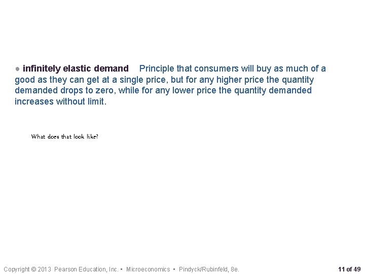
● infinitely elastic demand Principle that consumers will buy as much of a good as they can get at a single price, but for any higher price the quantity demanded drops to zero, while for any lower price the quantity demanded increases without limit. What does that look like? Copyright © 2013 Pearson Education, Inc. • Microeconomics • Pindyck/Rubinfeld, 8 e. 11 of 49

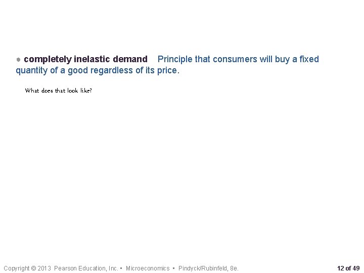
● completely inelastic demand Principle that consumers will buy a fixed quantity of a good regardless of its price. What does that look like? Copyright © 2013 Pearson Education, Inc. • Microeconomics • Pindyck/Rubinfeld, 8 e. 12 of 49

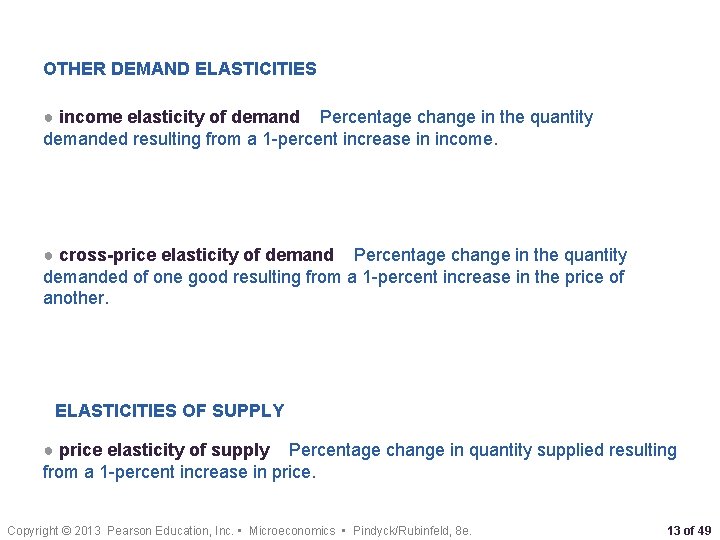
OTHER DEMAND ELASTICITIES ● income elasticity of demand Percentage change in the quantity demanded resulting from a 1 -percent increase in income. ● cross-price elasticity of demand Percentage change in the quantity demanded of one good resulting from a 1 -percent increase in the price of another. ELASTICITIES OF SUPPLY ● price elasticity of supply Percentage change in quantity supplied resulting from a 1 -percent increase in price. Copyright © 2013 Pearson Education, Inc. • Microeconomics • Pindyck/Rubinfeld, 8 e. 13 of 49

EXAMPLE 2. 5 BACK TO THE MARKET FOR WHEAT How much does quantity change when we change price by one dollar in our wheat equation? QD = 3550 − 266 P We use the demand curve to find the price elasticity of demand: Thus demand is inelastic. We can likewise calculate the price elasticity of supply: Because these supply and demand curves are linear, the price elasticities will vary as we move along the curves. Copyright © 2013 Pearson Education, Inc. • Microeconomics • Pindyck/Rubinfeld, 8 e. 14 of 49

Classwork 1. ) In the market for beers on a Tuesday night at the local bar, demand is represented by Qd=30 -5. 5 P and supply is Qs=1+. 75 P. Find the equilibrium price and quantity. 2. ) Find the price elasticity of demand supply at that equilibrium. 3. ) What is the elasticity of demand if price were $3? What’s the elasticity of supply at p=$3? What do those numbers mean? Copyright © 2013 Pearson Education, Inc. • Microeconomics • Pindyck/Rubinfeld, 8 e. 15 of 49

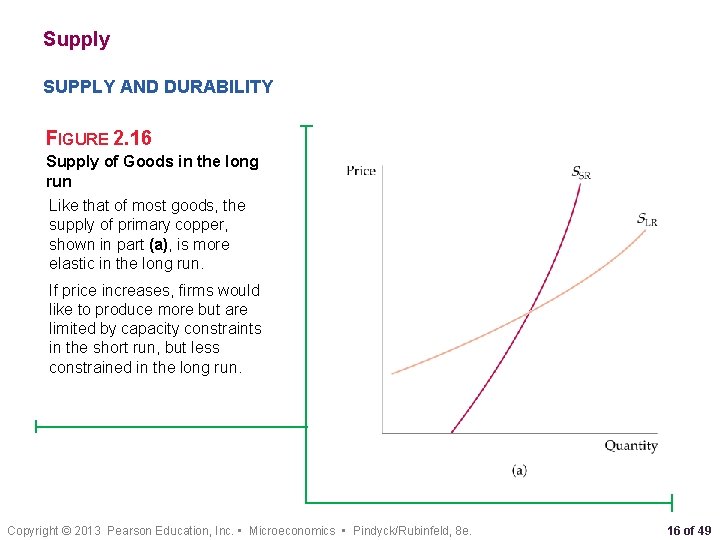
Supply SUPPLY AND DURABILITY FIGURE 2. 16 Supply of Goods in the long run Like that of most goods, the supply of primary copper, shown in part (a), is more elastic in the long run. If price increases, firms would like to produce more but are limited by capacity constraints in the short run, but less constrained in the long run. Copyright © 2013 Pearson Education, Inc. • Microeconomics • Pindyck/Rubinfeld, 8 e. 16 of 49

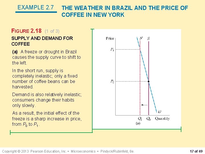
EXAMPLE 2. 7 FIGURE 2. 18 THE WEATHER IN BRAZIL AND THE PRICE OF COFFEE IN NEW YORK (1 of 3) SUPPLY AND DEMAND FOR COFFEE (a) A freeze or drought in Brazil causes the supply curve to shift to the left. In the short run, supply is completely inelastic; only a fixed number of coffee beans can be harvested. Demand is also relatively inelastic; consumers change their habits only slowly. As a result, the initial effect of the freeze is a sharp increase in price, from P 0 to P 1. Copyright © 2013 Pearson Education, Inc. • Microeconomics • Pindyck/Rubinfeld, 8 e. 17 of 49

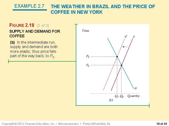
EXAMPLE 2. 7 FIGURE 2. 18 THE WEATHER IN BRAZIL AND THE PRICE OF COFFEE IN NEW YORK (2 of 3) SUPPLY AND DEMAND FOR COFFEE (b) In the intermediate run, supply and demand are both more elastic; thus price falls part of the way back, to P 2. Copyright © 2013 Pearson Education, Inc. • Microeconomics • Pindyck/Rubinfeld, 8 e. 18 of 49

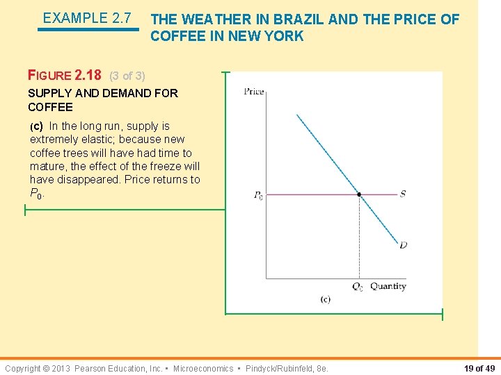
EXAMPLE 2. 7 FIGURE 2. 18 THE WEATHER IN BRAZIL AND THE PRICE OF COFFEE IN NEW YORK (3 of 3) SUPPLY AND DEMAND FOR COFFEE (c) In the long run, supply is extremely elastic; because new coffee trees will have had time to mature, the effect of the freeze will have disappeared. Price returns to P 0. Copyright © 2013 Pearson Education, Inc. • Microeconomics • Pindyck/Rubinfeld, 8 e. 19 of 49

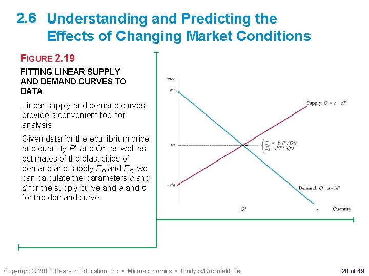
2. 6 Understanding and Predicting the Effects of Changing Market Conditions FIGURE 2. 19 FITTING LINEAR SUPPLY AND DEMAND CURVES TO DATA Linear supply and demand curves provide a convenient tool for analysis. Given data for the equilibrium price and quantity P* and Q*, as well as estimates of the elasticities of demand supply ED and ES, we can calculate the parameters c and d for the supply curve and a and b for the demand curve. Copyright © 2013 Pearson Education, Inc. • Microeconomics • Pindyck/Rubinfeld, 8 e. 20 of 49

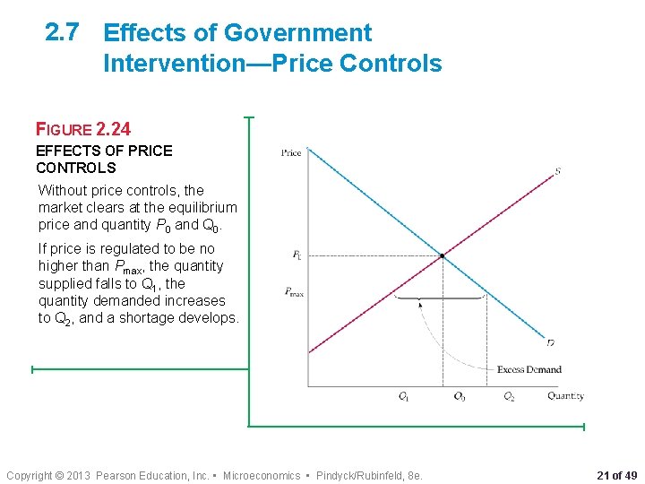
2. 7 Effects of Government Intervention—Price Controls FIGURE 2. 24 EFFECTS OF PRICE CONTROLS Without price controls, the market clears at the equilibrium price and quantity P 0 and Q 0. If price is regulated to be no higher than Pmax, the quantity supplied falls to Q 1, the quantity demanded increases to Q 2, and a shortage develops. Copyright © 2013 Pearson Education, Inc. • Microeconomics • Pindyck/Rubinfeld, 8 e. 21 of 49

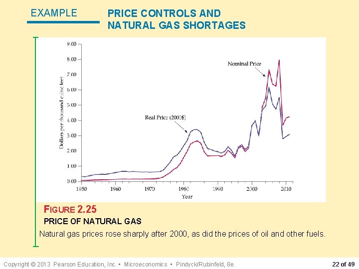
EXAMPLE PRICE CONTROLS AND NATURAL GAS SHORTAGES FIGURE 2. 25 PRICE OF NATURAL GAS Natural gas prices rose sharply after 2000, as did the prices of oil and other fuels. Copyright © 2013 Pearson Education, Inc. • Microeconomics • Pindyck/Rubinfeld, 8 e. 22 of 49

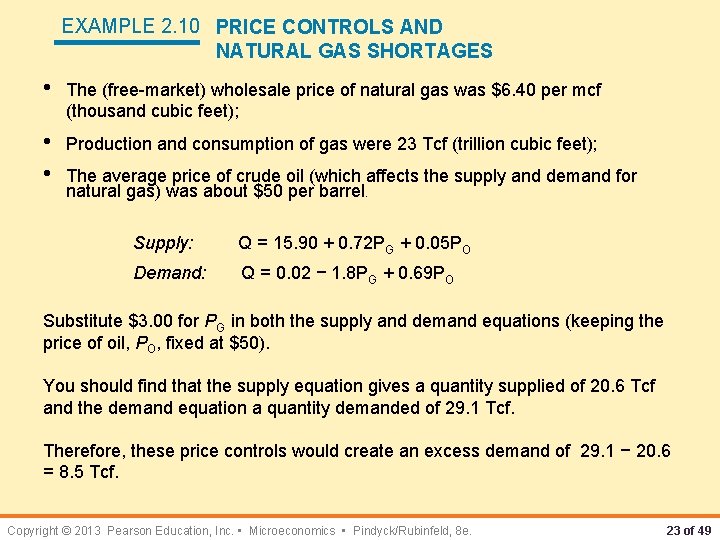
EXAMPLE 2. 10 PRICE CONTROLS AND NATURAL GAS SHORTAGES • The (free-market) wholesale price of natural gas was $6. 40 per mcf (thousand cubic feet); • • Production and consumption of gas were 23 Tcf (trillion cubic feet); The average price of crude oil (which affects the supply and demand for natural gas) was about $50 per barrel. Supply: Q = 15. 90 + 0. 72 PG + 0. 05 PO Demand: Q = 0. 02 − 1. 8 PG + 0. 69 PO Substitute $3. 00 for PG in both the supply and demand equations (keeping the price of oil, PO, fixed at $50). You should find that the supply equation gives a quantity supplied of 20. 6 Tcf and the demand equation a quantity demanded of 29. 1 Tcf. Therefore, these price controls would create an excess demand of 29. 1 − 20. 6 = 8. 5 Tcf. Copyright © 2013 Pearson Education, Inc. • Microeconomics • Pindyck/Rubinfeld, 8 e. 23 of 49