170 FIELD MAPPING V Blackmore CM 38 23

1/70 FIELD MAPPING V. Blackmore CM 38 23 rd February 2014

2/70 There is a lot of information in these slides, and not enough time to say it all. A lot of this will be revisited in future analysis meetings. I have added notes to most slides (if you download the. ppt version), so they should be understandable “offline. ” As for now, we’ll see just how far we get. . .

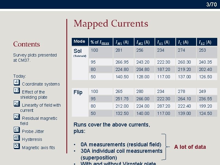
3/70 Mapped Currents Contents Survey plots presented at CM 37. Today: 4 Coordinate systems 17 Effect of the q q shielding plate 24 Linearity of field with q current q 29 Residual magnetic field 41 Probe Jitter q 48 q Hysteresis 50 q Magnetic axis fits Mode Sol 100 281 256 234 274 253 95 266. 95 243. 20 222. 30 260. 30 240. 35 80 224. 80 204. 80 187. 20 219. 20 202. 40 50 140. 50 128. 00 117. 00 137. 00 126. 50 100 265 280 234 278 249 95 251. 75 266. 00 222. 30 264. 10 236. 55 80 212. 00 224. 00 287. 20 222. 40 199. 20 50 132. 50 140. 00 117. 00 139. 00 124. 50 (Solenoid) Flip Runs cover the above currents, plus: • 0 A measurements (residual field) • 30 A individual coil measurements (superposition) A lot of data

4/70 COORDINATE SYSTEMS Until the end of this talk. . .

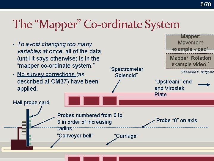
5/70 The “Mapper” Co-ordinate System Mapper: Movement example video* • To avoid changing too many variables at once, all of the data (until it says otherwise) is in the “mapper co-ordinate system. ” • No survey corrections (as described at CM 37) have been applied. “Spectrometer Solenoid” Mapper: Rotation example video * *Thanks to F. Bergsma “Upstream” end and Virostek Plate Hall probe card Probes numbered from 0 to 6 in order of increasing radius “Conveyor belt” “Carriage” Probe “ 0” on axis

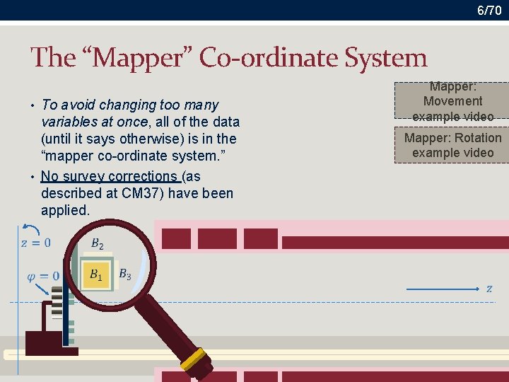
6/70 The “Mapper” Co-ordinate System • To avoid changing too many variables at once, all of the data (until it says otherwise) is in the “mapper co-ordinate system. ” • No survey corrections (as described at CM 37) have been applied. Mapper: Movement example video Mapper: Rotation example video

7/70 The “Mapper” Co-ordinate System • To avoid changing too many variables at once, all of the data (until it says otherwise) is in the “mapper co-ordinate system. ” • No survey corrections (as described at CM 37) have been applied. Tick! Mapper: Movement example video Mapper: Rotation example video

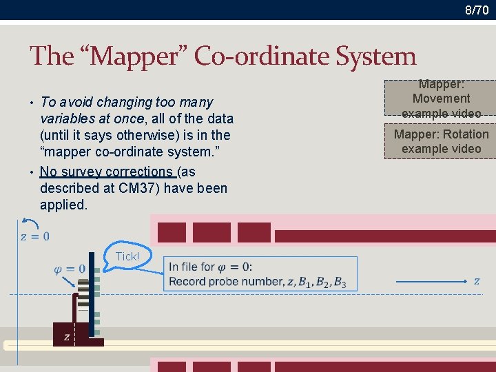
8/70 The “Mapper” Co-ordinate System • To avoid changing too many variables at once, all of the data (until it says otherwise) is in the “mapper co-ordinate system. ” • No survey corrections (as described at CM 37) have been applied. Tick! Mapper: Movement example video Mapper: Rotation example video

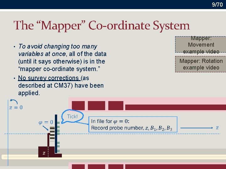
9/70 The “Mapper” Co-ordinate System • To avoid changing too many variables at once, all of the data (until it says otherwise) is in the “mapper co-ordinate system. ” • No survey corrections (as described at CM 37) have been applied. Tick! Mapper: Movement example video Mapper: Rotation example video

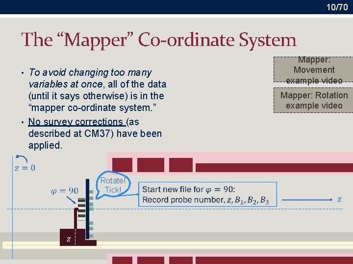
10/70 The “Mapper” Co-ordinate System • To avoid changing too many variables at once, all of the data (until it says otherwise) is in the “mapper co-ordinate system. ” • No survey corrections (as described at CM 37) have been applied. Rotate! Tick! Mapper: Movement example video Mapper: Rotation example video

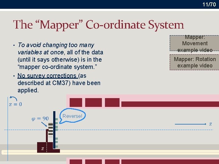
11/70 The “Mapper” Co-ordinate System • To avoid changing too many variables at once, all of the data (until it says otherwise) is in the “mapper co-ordinate system. ” • No survey corrections (as described at CM 37) have been applied. Reverse! Mapper: Movement example video Mapper: Rotation example video

12/70 The “Mapper” Co-ordinate System • To avoid changing too many variables at once, all of the data (until it says otherwise) is in the “mapper co-ordinate system. ” • No survey corrections (as described at CM 37) have been applied. Tick! Mapper: Movement example video Mapper: Rotation example video

13/70 The “Mapper” Co-ordinate System • To avoid changing too many variables at once, all of the data (until it says otherwise) is in the “mapper co-ordinate system. ” • No survey corrections (as described at CM 37) have been applied. Tick! Mapper: Movement example video Mapper: Rotation example video

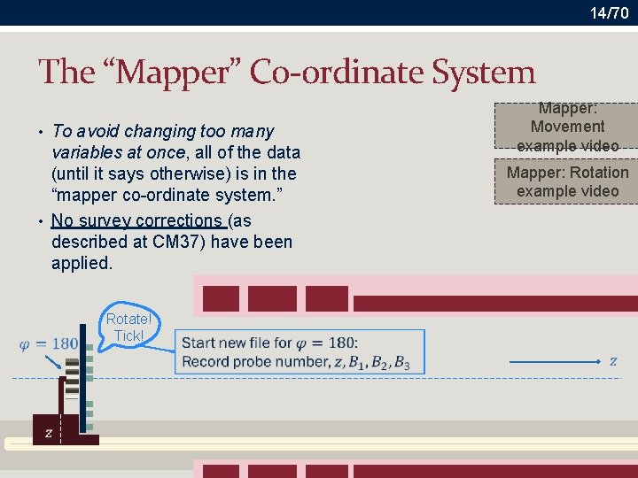
14/70 The “Mapper” Co-ordinate System • To avoid changing too many variables at once, all of the data (until it says otherwise) is in the “mapper co-ordinate system. ” • No survey corrections (as described at CM 37) have been applied. Rotate! Tick! Mapper: Movement example video Mapper: Rotation example video

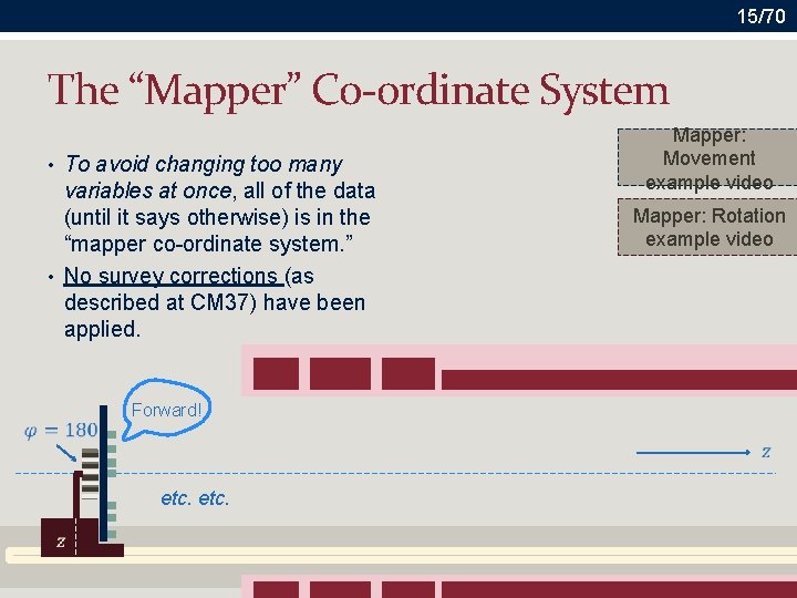
15/70 The “Mapper” Co-ordinate System • To avoid changing too many variables at once, all of the data (until it says otherwise) is in the “mapper co-ordinate system. ” • No survey corrections (as described at CM 37) have been applied. Forward! etc. Mapper: Movement example video Mapper: Rotation example video

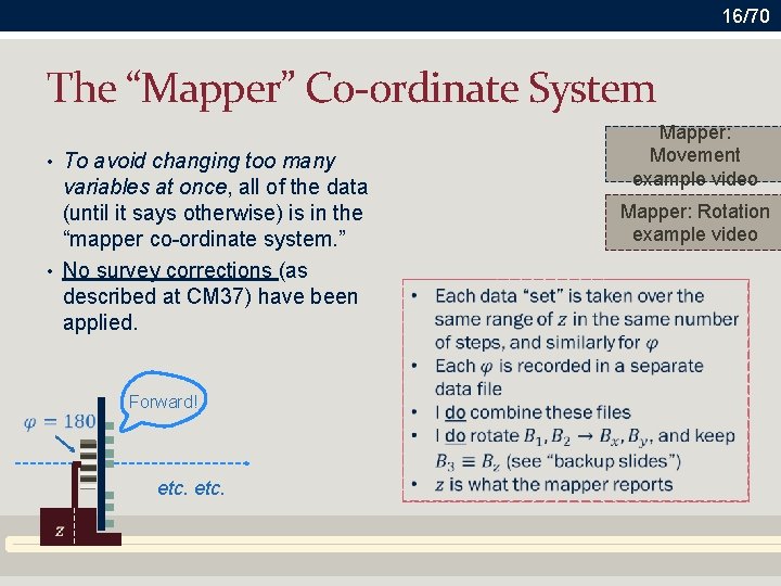
16/70 The “Mapper” Co-ordinate System • To avoid changing too many variables at once, all of the data (until it says otherwise) is in the “mapper co-ordinate system. ” • No survey corrections (as described at CM 37) have been applied. Forward! etc. Mapper: Movement example video Mapper: Rotation example video

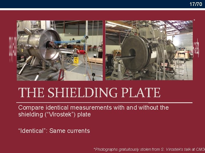
17/70 * THE SHIELDING PLATE Compare identical measurements with and without the shielding (“Virostek”) plate “Identical”: Same currents *Photographs gratuitously stolen from S. Virostek’s talk at CM 36

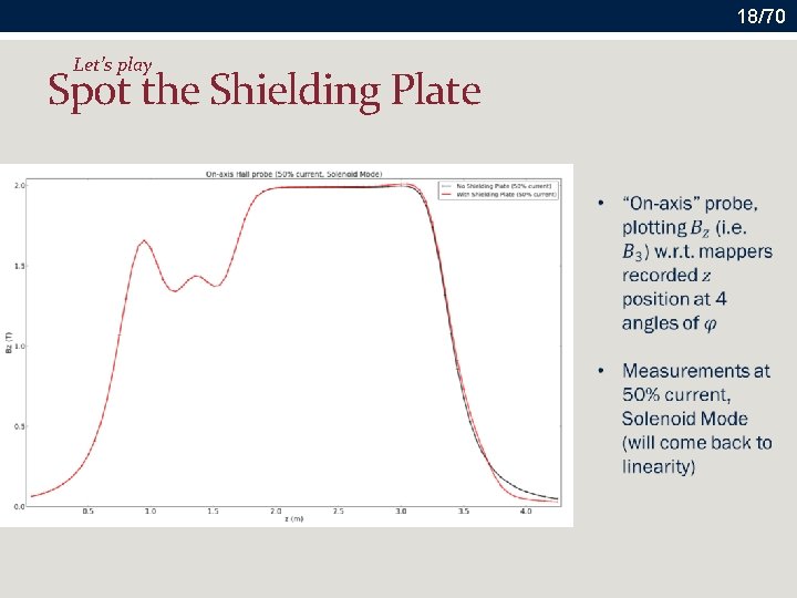
18/70 Let’s play Spot the Shielding Plate

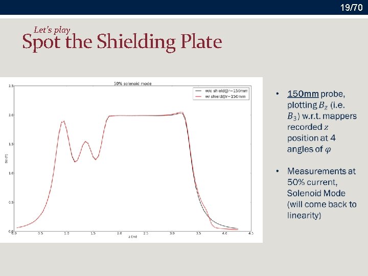
19/70 Let’s play Spot the Shielding Plate

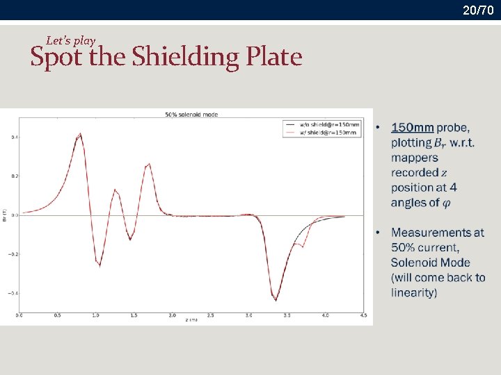
20/70 Let’s play Spot the Shielding Plate

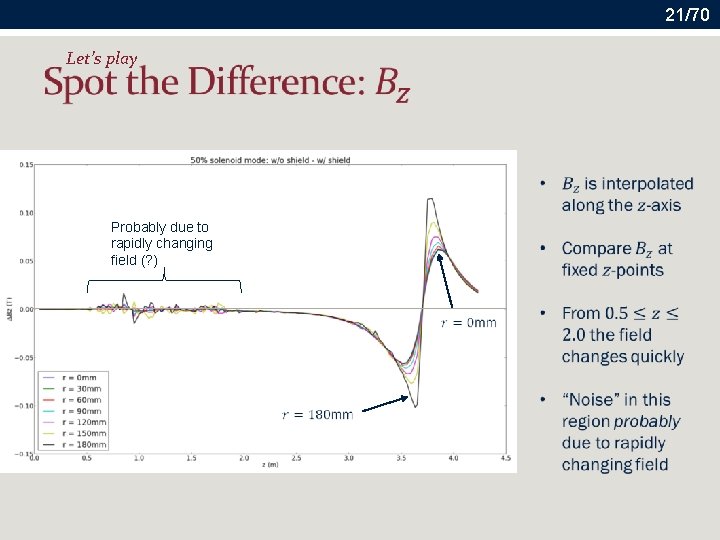
21/70 Let’s play Probably due to rapidly changing field (? )

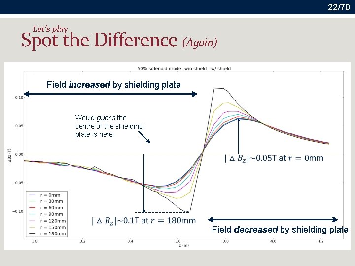
22/70 Let’s play Spot the Difference (Again) Field increased by shielding plate Would guess the centre of the shielding plate is here! Field decreased by shielding plate

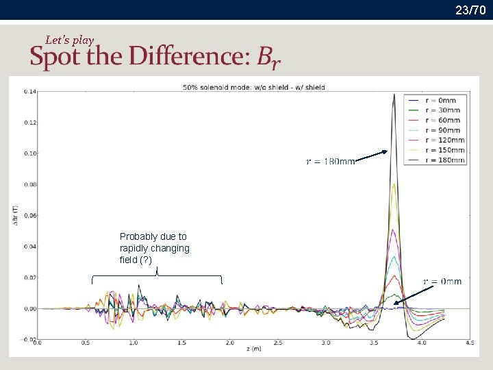
23/70 Let’s play Probably due to rapidly changing field (? )

24/70 FIELD LINEARITY With no shielding plate, field should be linear with current. With shielding plate, field may be non-linear with current

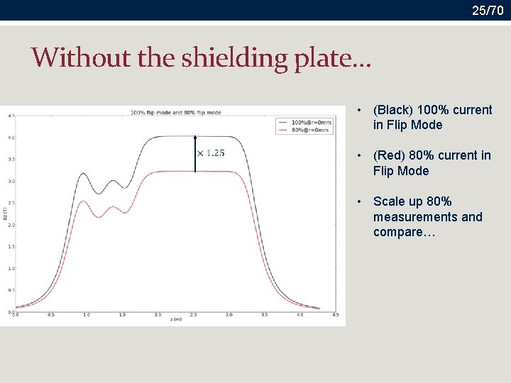
25/70 Without the shielding plate… • (Black) 100% current in Flip Mode • (Red) 80% current in Flip Mode • Scale up 80% measurements and compare…

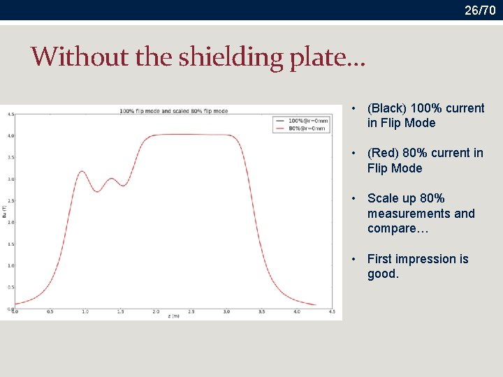
26/70 Without the shielding plate… • (Black) 100% current in Flip Mode • (Red) 80% current in Flip Mode • Scale up 80% measurements and compare… • First impression is good.

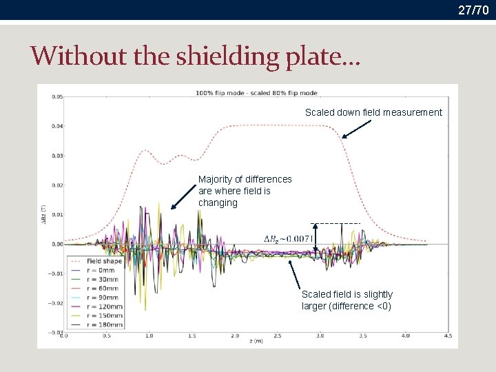
27/70 Without the shielding plate… Scaled down field measurement Majority of differences are where field is changing Scaled field is slightly larger (difference <0)

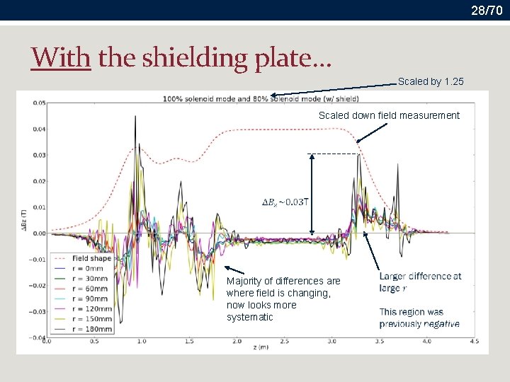
28/70 With the shielding plate… Scaled by 1. 25 Scaled down field measurement Majority of differences are where field is changing, now looks more systematic

29/70 RESIDUAL FIELD We do have data sets that allow us to naively look at the residual field Q: Does the residual field change depending on the previous operating current?

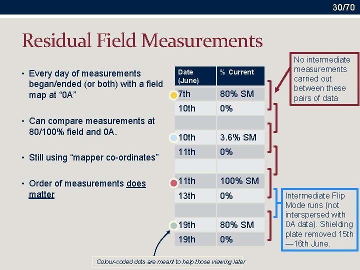
30/70 Residual Field Measurements • Every day of measurements began/ended (or both) with a field map at “ 0 A” Date (June) % Current 7 th 80% SM 10 th 0% 10 th 3. 6% SM 11 th 0% 11 th 100% SM 13 th 0% 19 th 80% SM 19 th 0% No intermediate measurements carried out between these pairs of data • Can compare measurements at 80/100% field and 0 A. • Still using “mapper co-ordinates” • Order of measurements does matter Colour-coded dots are meant to help those viewing later Intermediate Flip Mode runs (not interspersed with 0 A data). Shielding plate removed 15 th — 16 th June.

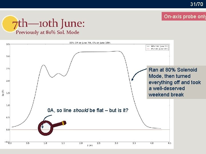
31/70 7 th— 10 th June: On-axis probe only Previously at 80% Sol. Mode Ran at 80% Solenoid Mode, then turned everything off and took a well-deserved weekend break 0 A, so line should be flat – but is it?

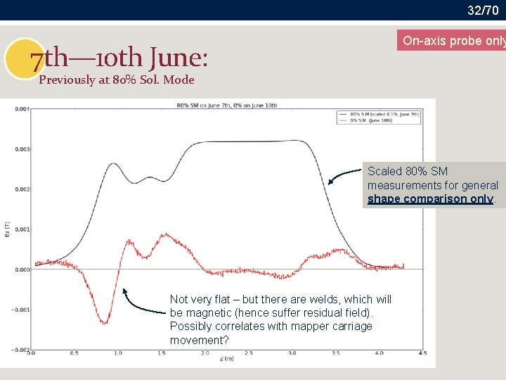
32/70 On-axis probe only 7 th— 10 th June: Previously at 80% Sol. Mode Scaled 80% SM measurements for general shape comparison only. Not very flat – but there are welds, which will be magnetic (hence suffer residual field). Possibly correlates with mapper carriage movement?

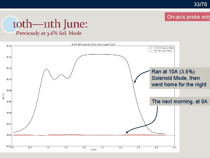
33/70 10 th— 11 th June: On-axis probe only Previously at 3. 6% Sol. Mode Ran at 10 A (3. 6%) Solenoid Mode, then went home for the night The next morning, at 0 A

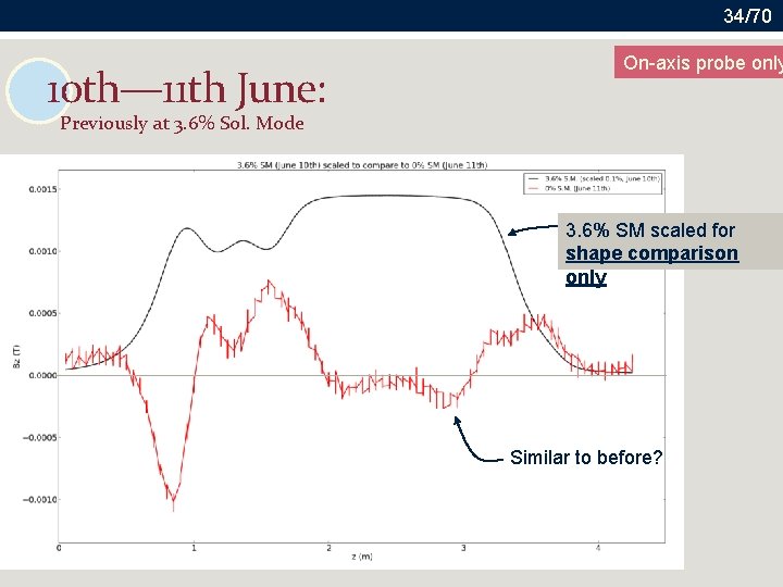
34/70 10 th— 11 th June: On-axis probe only Previously at 3. 6% Sol. Mode 3. 6% SM scaled for shape comparison only Similar to before?

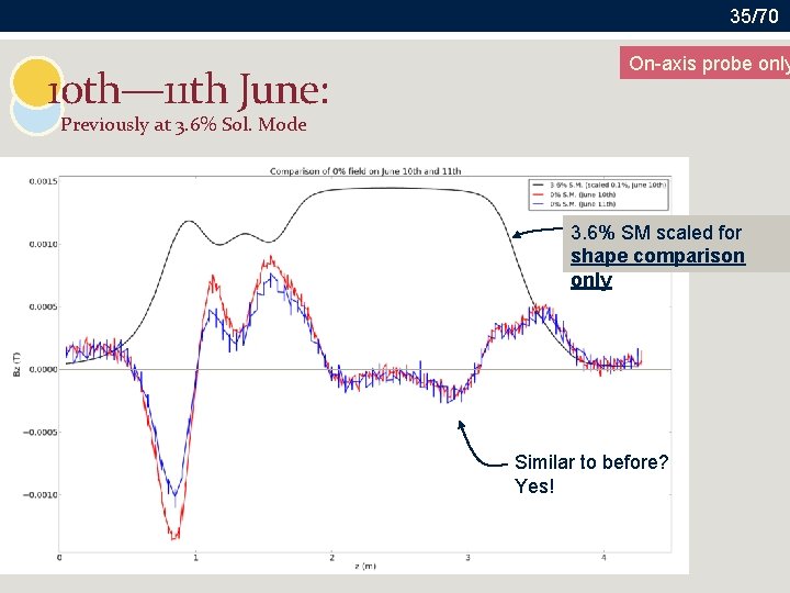
35/70 10 th— 11 th June: On-axis probe only Previously at 3. 6% Sol. Mode 3. 6% SM scaled for shape comparison only Similar to before? Yes!

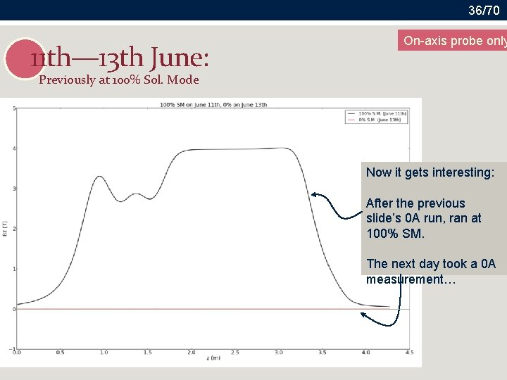
36/70 11 th— 13 th June: On-axis probe only Previously at 100% Sol. Mode Now it gets interesting: After the previous slide’s 0 A run, ran at 100% SM. The next day took a 0 A measurement…

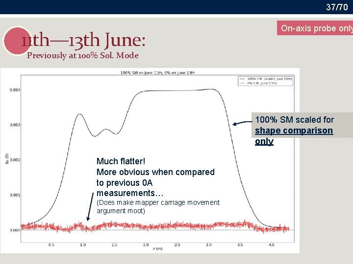
37/70 11 th— 13 th June: On-axis probe only Previously at 100% Sol. Mode 100% SM scaled for shape comparison only Much flatter! More obvious when compared to previous 0 A measurements… (Does make mapper carriage movement argument moot)

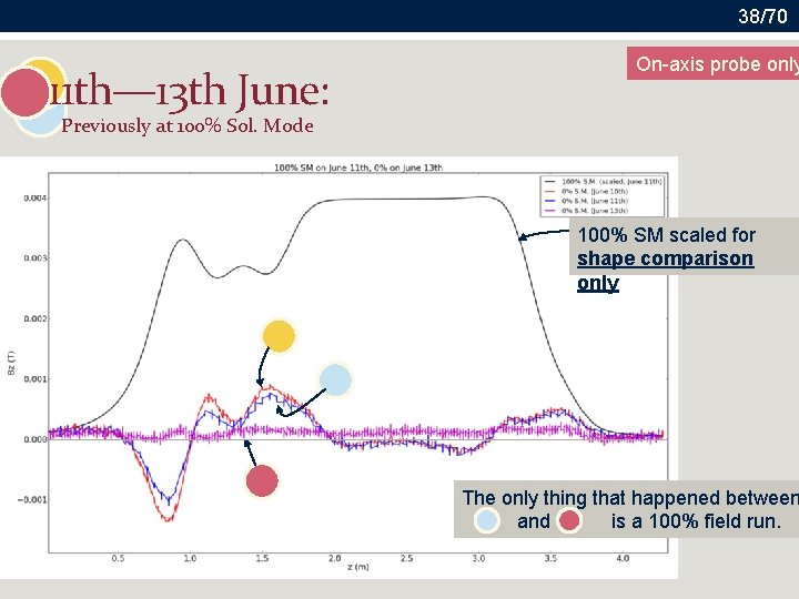
38/70 11 th— 13 th June: On-axis probe only Previously at 100% Sol. Mode 100% SM scaled for shape comparison only The only thing that happened between and is a 100% field run.

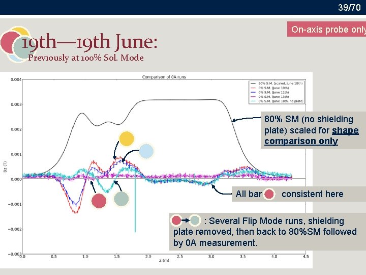
39/70 On-axis probe only 19 th— 19 th June: Previously at 100% Sol. Mode 80% SM (no shielding plate) scaled for shape comparison only All bar consistent here : Several Flip Mode runs, shielding plate removed, then back to 80%SM followed by 0 A measurement.

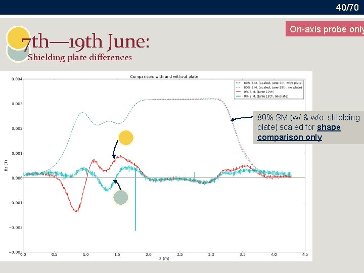
40/70 7 th— 19 th June: On-axis probe only Shielding plate differences 80% SM (w/ & w/o shielding plate) scaled for shape comparison only

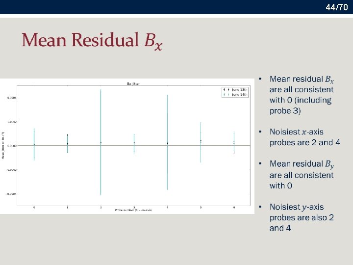
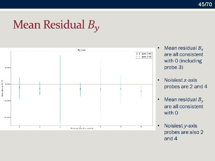
41/70 PROBE JITTER What kind of error bars should we be imagining on the previous plots? Look at the “flat” regions of the 0 A measurements and see what variation there is in probe readout.

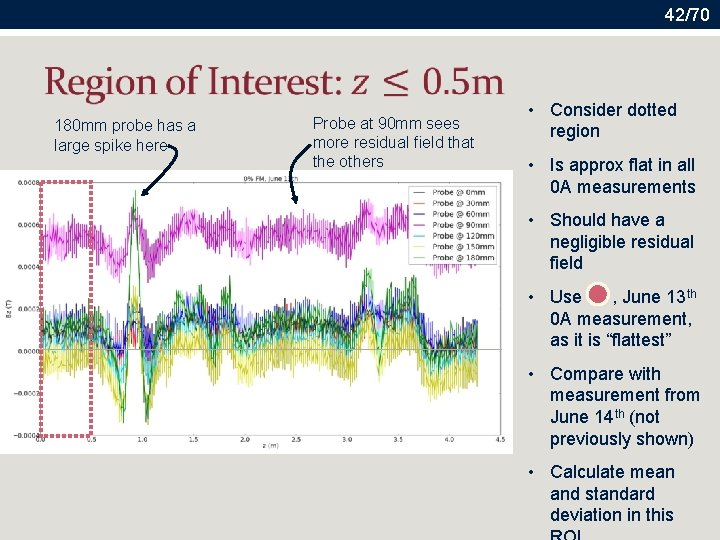
42/70 180 mm probe has a large spike here Probe at 90 mm sees more residual field that the others • Consider dotted region • Is approx flat in all 0 A measurements • Should have a negligible residual field • Use , June 13 th 0 A measurement, as it is “flattest” • Compare with measurement from June 14 th (not previously shown) • Calculate mean and standard deviation in this

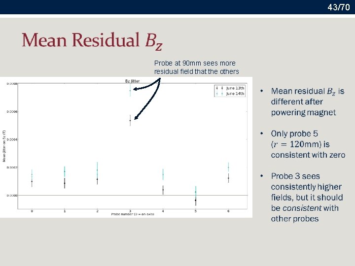
43/70 Probe at 90 mm sees more residual field that the others

44/70

45/70

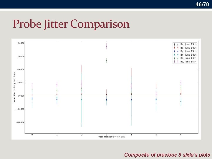
46/70 Probe Jitter Comparison Composite of previous 3 slide’s plots

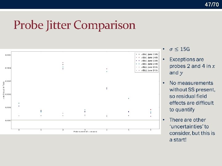
47/70 Probe Jitter Comparison

48/70 HYSTERESIS Q: Do we achieve the same field when we approach it from below the operating current and above the operating current?

49/70 Hysteresis • Ideally, requires consecutive four measurements with the shielding plate • 0% solenoid/flip • 80% solenoid/flip mode • 100% solenoid/flip mode • 80% solenoid/flip mode • We have 0% 80%, and 0% 100%, but do not have 100% 80% • Mapping takes a long time • Time taken by shielding plate installation and removal • Judging by changes in residual field, likely there will be a (very) small hysteresis effect • Should make this measurement when mapping final SS

50/70 FINDING THE MAGNETIC AXIS (FIRST PASS) The mapper moves about by ~ 1 mm in (x, y) as it travels through the magnet To first approximation, ignore this movement and use mapper coordinates to get an estimate of the magnetic axis

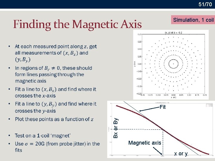
51/70 Finding the Magnetic Axis Simulation, 1 coil Bx or By Fit Magnetic axis x or y

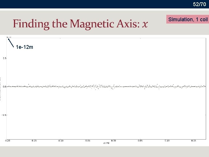
52/70 Simulation, 1 coil 1 e-12 m

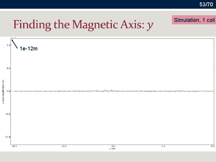
53/70 Simulation, 1 coil 1 e-12 m

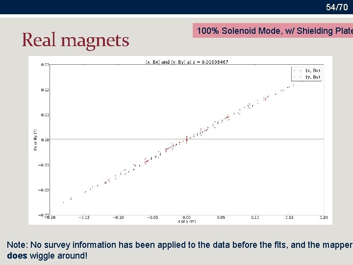
54/70 Real magnets 100% Solenoid Mode, w/ Shielding Plate Note: No survey information has been applied to the data before the fits, and the mapper does wiggle around!

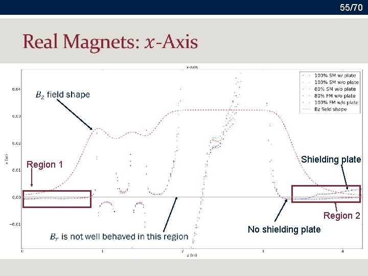
55/70 Region 1 Shielding plate Region 2 No shielding plate

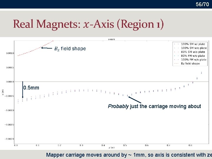
56/70 0. 5 mm Probably just the carriage moving about Mapper carriage moves around by ~ 1 mm, so axis is consistent with ze

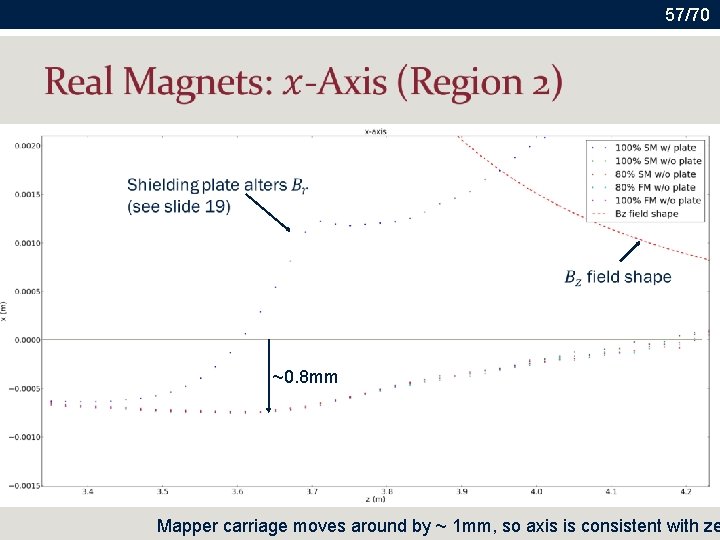
57/70 ~0. 8 mm Mapper carriage moves around by ~ 1 mm, so axis is consistent with ze

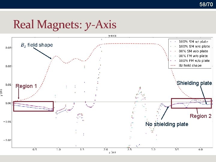
58/70 Region 1 Shielding plate Region 2 No shielding plate

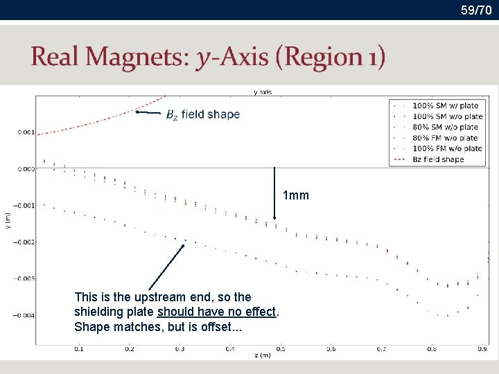
59/70 1 mm This is the upstream end, so the shielding plate should have no effect. Shape matches, but is offset. . .

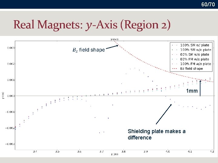
60/70 1 mm Shielding plate makes a difference

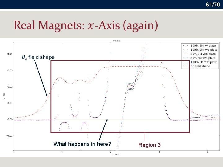
61/70 What happens in here? Region 3

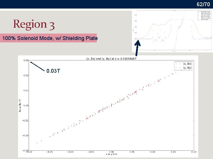
62/70 Region 3 100% Solenoid Mode, w/ Shielding Plate 0. 03 T

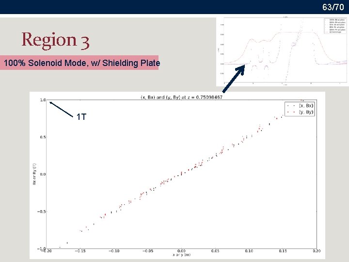
63/70 Region 3 100% Solenoid Mode, w/ Shielding Plate 1 T

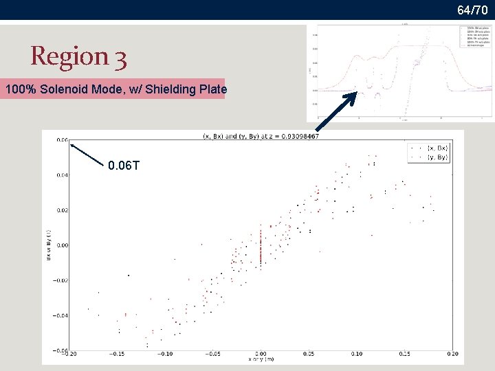
64/70 Region 3 100% Solenoid Mode, w/ Shielding Plate 0. 06 T

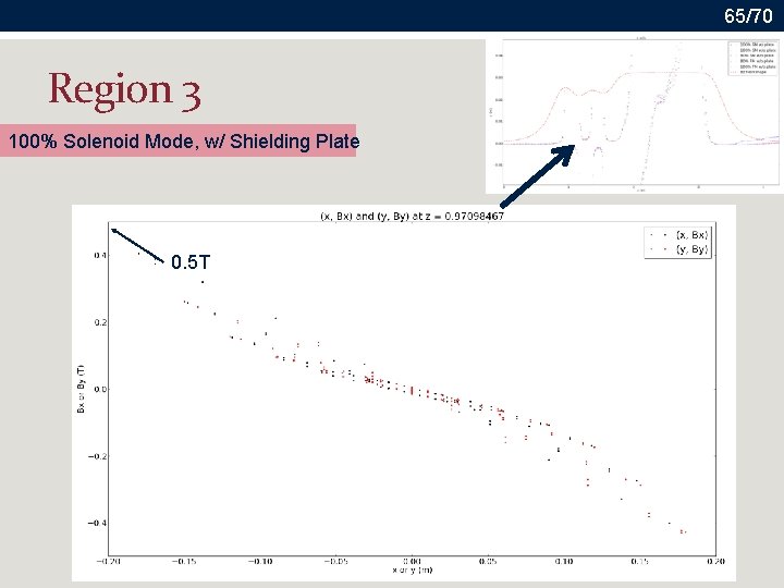
65/70 Region 3 100% Solenoid Mode, w/ Shielding Plate 0. 5 T

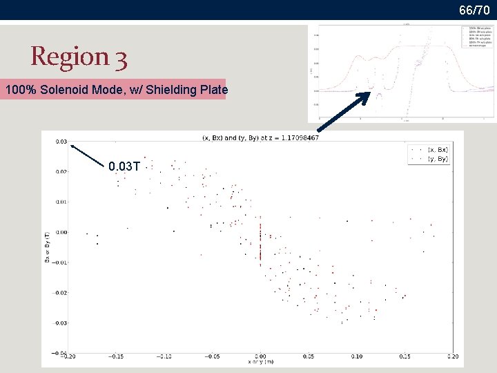
66/70 Region 3 100% Solenoid Mode, w/ Shielding Plate 0. 03 T

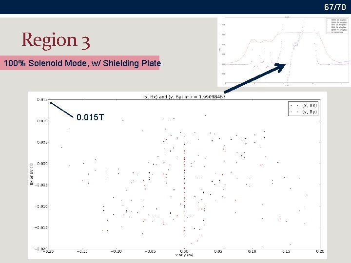
67/70 Region 3 100% Solenoid Mode, w/ Shielding Plate 0. 015 T

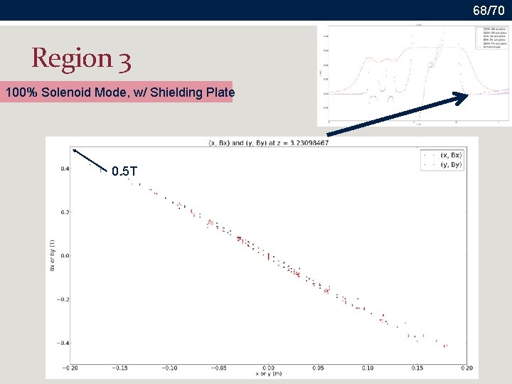
68/70 Region 3 100% Solenoid Mode, w/ Shielding Plate 0. 5 T

CONCLUSIONS

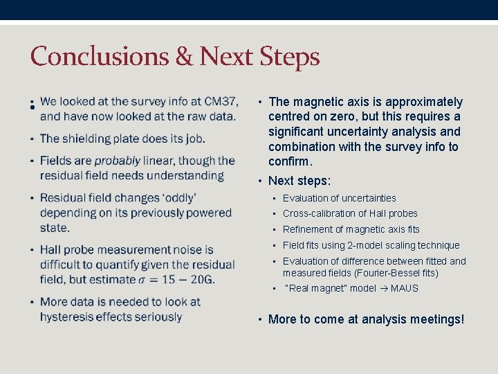
Conclusions & Next Steps • • The magnetic axis is approximately centred on zero, but this requires a significant uncertainty analysis and combination with the survey info to confirm. • Next steps: • Evaluation of uncertainties • Cross-calibration of Hall probes • Refinement of magnetic axis fits • Field fits using 2 -model scaling technique • Evaluation of difference between fitted and measured fields (Fourier-Bessel fits) • “Real magnet” model MAUS • More to come at analysis meetings!

BACK-UP SLIDES A. Interpolation reliability B. Mapper co-ordinate transforms

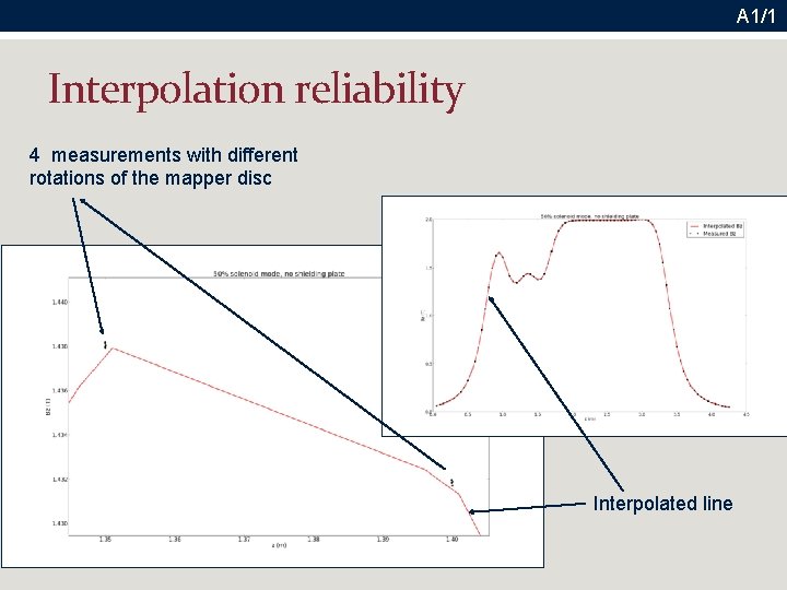
A 1/1 Interpolation reliability 4 measurements with different rotations of the mapper disc Interpolated line

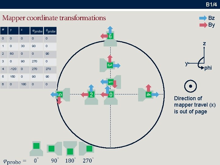
B 1/4 Mapper co 0 rdinate transformations y z 0 0 0 1 0 30 90 0 2 60 0 0 90 3 0 90 270 0 4 -120 0 270 5 150 0 90 90 6 0 180 0 0 6 z y phi 2 0 4 5 1 3 # Bz By Direction of mapper travel (x) is out of page

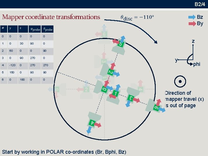
B 2/4 Mapper co 0 rdinate transformations y z 0 0 0 1 0 30 90 0 2 60 0 0 90 3 0 90 270 0 4 -120 0 270 5 150 0 90 90 6 0 180 0 0 6 z 5 y 3 # Bz By phi 3 1 4 5 1 2 0 0 2 6 4 Start by working in POLAR co-ordinates (Br, Bphi, Bz) Direction of mapper travel (x) is out of page

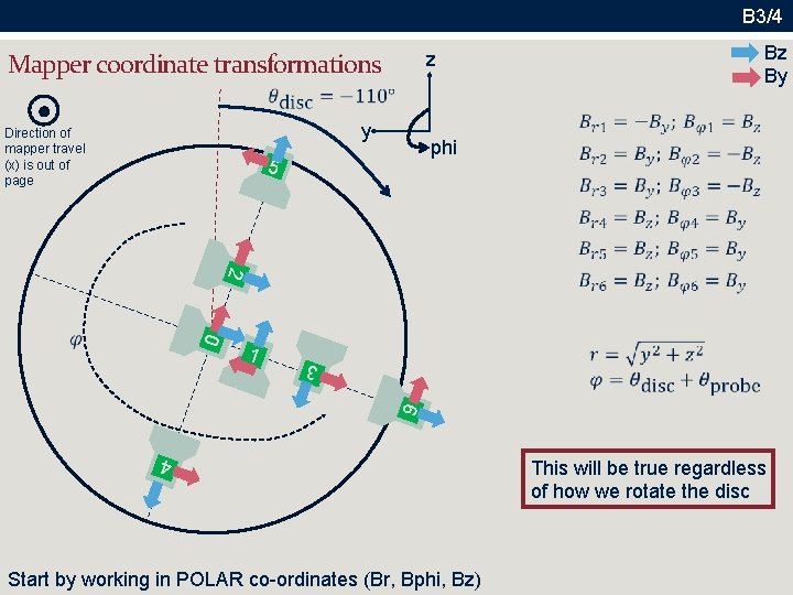
B 3/4 z Mapper co 0 rdinate transformations y Direction of mapper travel (x) is out of page Bz By phi 5 2 3 0 1 6 4 Start by working in POLAR co-ordinates (Br, Bphi, Bz) This will be true regardless of how we rotate the disc

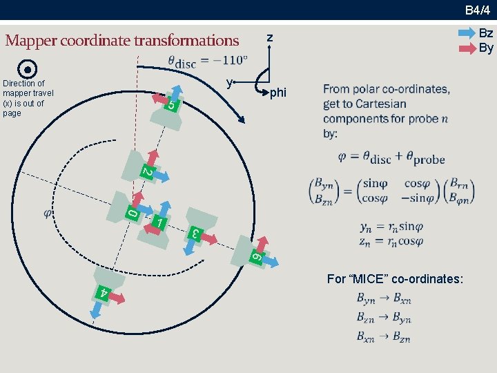
B 4/4 y Direction of mapper travel (x) is out of page Bz By z Mapper co 0 rdinate transformations phi 5 2 3 0 1 6 For “MICE” co-ordinates: 4