16 Risk Ratios 12202021 Risk ratios 1 Comparing

16: Risk Ratios 12/20/2021 Risk ratios 1

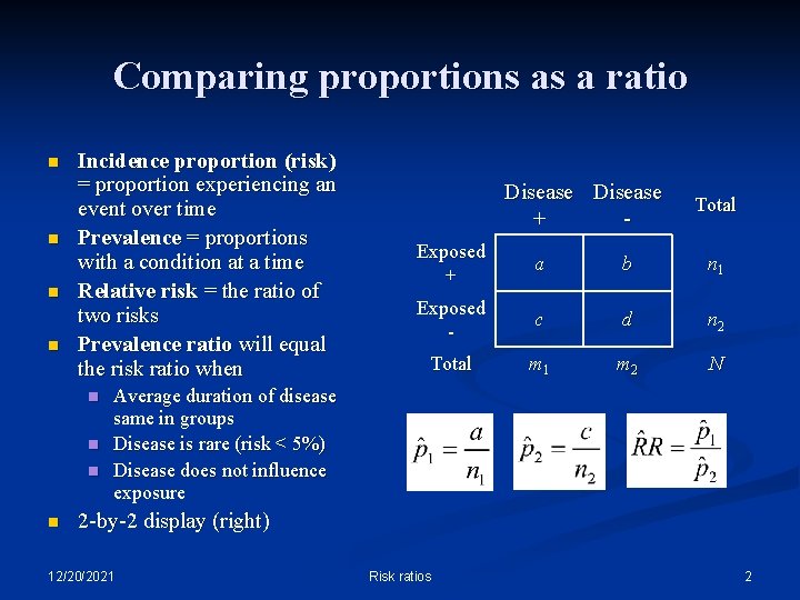
Comparing proportions as a ratio n n Incidence proportion (risk) = proportion experiencing an event over time Prevalence = proportions with a condition at a time Relative risk = the ratio of two risks Prevalence ratio will equal the risk ratio when n n Disease + - Total Exposed + a b n 1 Exposed - c d n 2 Total m 1 m 2 N Average duration of disease same in groups Disease is rare (risk < 5%) Disease does not influence exposure 2 -by-2 display (right) 12/20/2021 Risk ratios 2

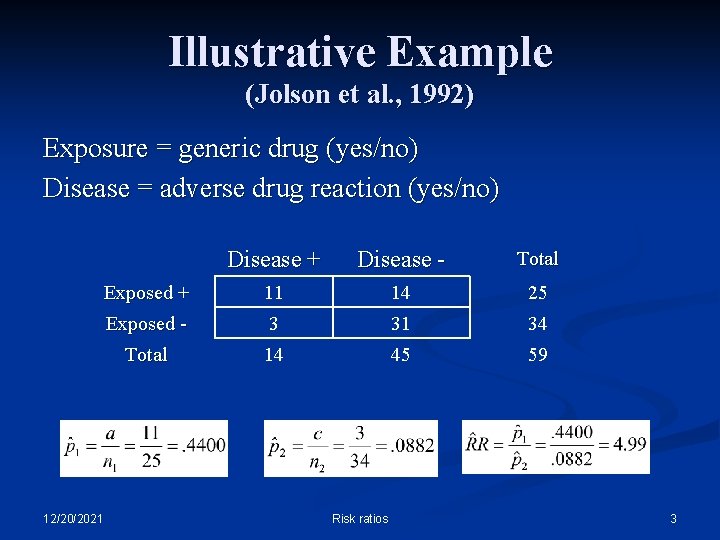
Illustrative Example (Jolson et al. , 1992) Exposure = generic drug (yes/no) Disease = adverse drug reaction (yes/no) 12/20/2021 Disease + Disease - Total Exposed + 11 14 25 Exposed - 3 31 34 Total 14 45 59 Risk ratios 3

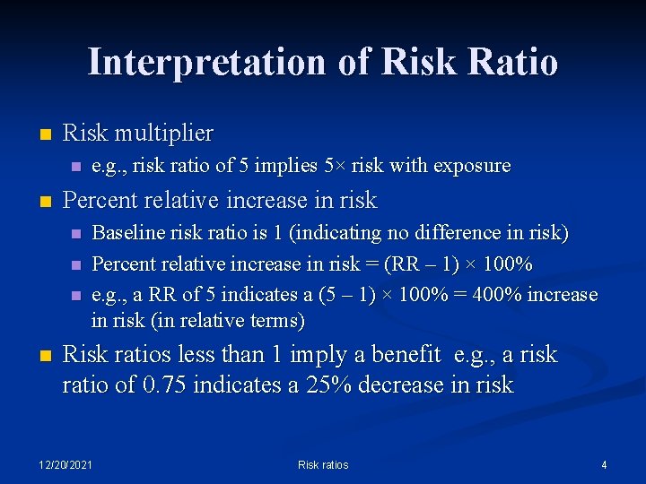
Interpretation of Risk Ratio n Risk multiplier n n Percent relative increase in risk n n e. g. , risk ratio of 5 implies 5× risk with exposure Baseline risk ratio is 1 (indicating no difference in risk) Percent relative increase in risk = (RR – 1) × 100% e. g. , a RR of 5 indicates a (5 – 1) × 100% = 400% increase in risk (in relative terms) Risk ratios less than 1 imply a benefit e. g. , a risk ratio of 0. 75 indicates a 25% decrease in risk 12/20/2021 Risk ratios 4

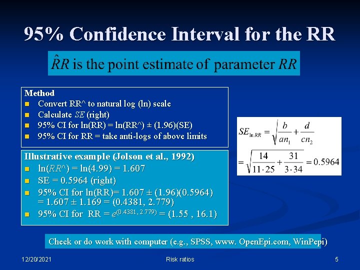
95% Confidence Interval for the RR Method n Convert RR^ to natural log (ln) scale n Calculate SE (right) n 95% CI for ln(RR) = ln(RR^) ± (1. 96)(SE) n 95% CI for RR = take anti-logs of above limits Illustrative example (Jolson et al. , 1992) n ln(RR^) = ln(4. 99) = 1. 607 n SE = 0. 5964 (right) n 95% CI for ln(RR)= 1. 607 ± (1. 96)(0. 5964) = 1. 607 ± 1. 169 = (0. 4381, 2. 779) n 95% CI for RR = e(0. 4381, 2. 779) = (1. 55 , 16. 1) Check or do work with computer (e. g. , SPSS, www. Open. Epi. com, Win. Pepi) 12/20/2021 Risk ratios 5

Confidence Interval n Locates parameter with “wiggle room” n n We are 95% confident RR is between 1. 55 and 16. 1 Confidence interval width quantifies precision of the estimate Wide imprecise estimate n Narrow precise estimate n 12/20/2021 Risk ratios 6

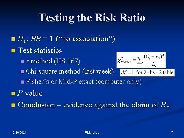
Testing the Risk Ratio H 0: RR = 1 (“no association”) n Test statistics n z method (HS 167) n Chi-square method (last week) n Fisher’s or Mid-P exact (computer only) n P value n Conclusion – evidence against the claim of H 0 n 12/20/2021 Risk ratios 7

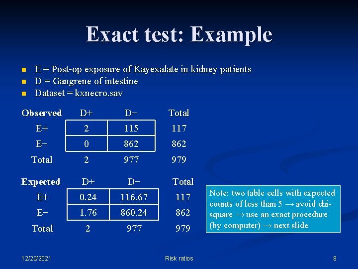
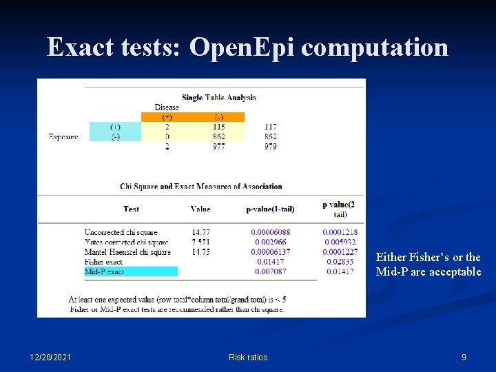
Exact test: Example n n n E = Post-op exposure of Kayexalate in kidney patients D = Gangrene of intestine Dataset = kxnecro. sav Observed D+ D− Total E+ 2 115 117 E− 0 862 Total 2 977 979 Expected D+ D− Total E+ 0. 24 116. 67 117 E− 1. 76 860. 24 862 Total 2 977 979 12/20/2021 Risk ratios Note: two table cells with expected counts of less than 5 → avoid chisquare → use an exact procedure (by computer) → next slide 8

Exact tests: Open. Epi computation Either Fisher’s or the Mid-P are acceptable 12/20/2021 Risk ratios 9

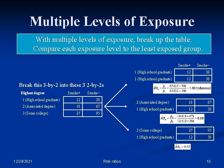
Multiple Levels of Exposure With multiple levels of exposure, break up the table. Compare each exposure level to the least exposed group. Smoke+ Smoke− 1 (High school graduate) 12 38 Break this 3 -by-2 into these 3 2 -by-2 s Highest degree Smoke+ Smoke− 1 (High school graduate) 12 38 2 (Associated degree) 18 67 3 (Some college) 27 95 12/20/2021 Risk ratios 2 (Associated degree) 18 67 1 (High school graduate) 12 38 3 (Some college) 27 95 1 (High school graduate) 12 38 10

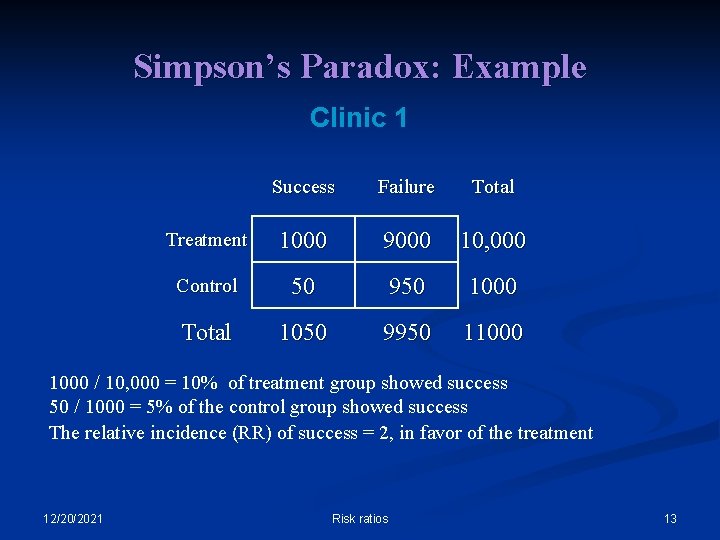
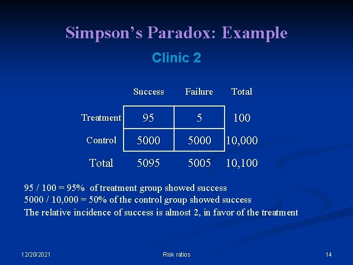
Simpson’s Paradox (Extreme confounding) Confounding a form of bias in which a lurking variable creates a spurious association between variables n Simpson’s paradox an extreme confounding in which the lurking variable creates a reversal in the direction of an association n 12/20/2021 Risk ratios 11

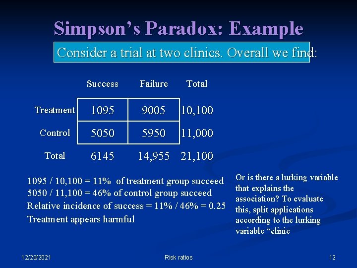
Simpson’s Paradox: Example Consider a trial at two clinics. Overall we find: Success Failure Total Treatment 1095 9005 10, 100 Control 5050 5950 11, 000 Total 6145 14, 955 21, 100 1095 / 10, 100 = 11% of treatment group succeed 5050 / 11, 100 = 46% of control group succeed Relative incidence of success = 11% / 46% = 0. 25 Treatment appears harmful 12/20/2021 Risk ratios Or is there a lurking variable that explains the association? To evaluate this, split applications according to the lurking variable “clinic 12

Simpson’s Paradox: Example Clinic 1 Success Failure Total Treatment 1000 9000 10, 000 Control 50 950 1000 Total 1050 9950 11000 / 10, 000 = 10% of treatment group showed success 50 / 1000 = 5% of the control group showed success The relative incidence (RR) of success = 2, in favor of the treatment 12/20/2021 Risk ratios 13

Simpson’s Paradox: Example Clinic 2 Success Failure Total Treatment 95 5 100 Control 5000 10, 000 Total 5095 5005 10, 100 95 / 100 = 95% of treatment group showed success 5000 / 10, 000 = 50% of the control group showed success The relative incidence of success is almost 2, in favor of the treatment 12/20/2021 Risk ratios 14

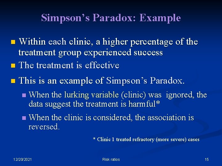
Simpson’s Paradox: Example Within each clinic, a higher percentage of the treatment group experienced success n The treatment is effective n n This is an example of Simpson’s Paradox. n When the lurking variable (clinic) was ignored, the data suggest the treatment is harmful* n When the clinic is considered, the association is reversed. * Clinic 1 treated refractory (more severe) cases 12/20/2021 Risk ratios 15

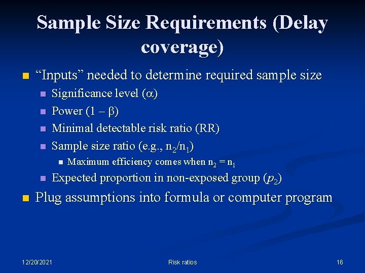
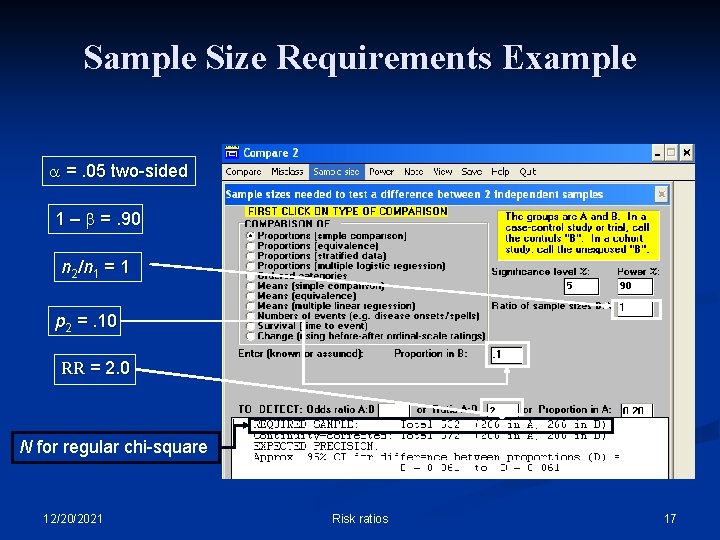
Sample Size Requirements (Delay coverage) n “Inputs” needed to determine required sample size n n Significance level (a) Power (1 – b) Minimal detectable risk ratio (RR) Sample size ratio (e. g. , n 2/n 1) n n n Maximum efficiency comes when n 2 = n 1 Expected proportion in non-exposed group (p 2) Plug assumptions into formula or computer program 12/20/2021 Risk ratios 16

Sample Size Requirements Example a =. 05 two-sided 1 – b =. 90 n 2 / n 1 = 1 p 2 =. 10 RR = 2. 0 N for regular chi-square 12/20/2021 Risk ratios 17