16 Odds Ratios from casecontrol studies Casecontrol studies

16: Odds Ratios [from case-control studies] Case-control studies get around several limitations of cohort studies

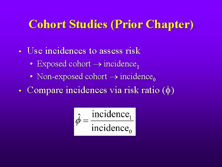
Cohort Studies (Prior Chapter) • Use incidences to assess risk • • • Exposed cohort incidence 1 Non-exposed cohort incidence 0 Compare incidences via risk ratio ( )

Hindrances in Cohort Studies • • Long induction between exposure & disease may cause delays Study of rare diseases require large sample sizes to accrue sufficient numbers When studying many people information by necessity can be limited in scope & accuracy Case-control studies were developed to help overcome some of these limitations

Levin et al. (1950) Historically important study (not in Reader) • Selection criteria • 236 lung cancer cases -- 156 (66%) smoked • 481 non-cancerous conditions (“controls”) -212 (44%) smoked • Although incidences of lung cancer cannot be determined from data, we see an association between smoking and lung cancer

How do we quantify risk from case -control data? • • Two article shed light on this question Cornfield, 1951 Cornfield, J. (1951). A method of estimating comparative rates from clinical data. Application to cancer of the lung, breast, and cervix. Journal of the National Cancer Institute, 11, 1269 -1275. • Miettinen, 1976 Miettinen, O. (1976). Estimability and estimation in case-referent studies. American Journal of Epidemiology, 103, 226 -235.

Cornfield, 1951 • • Justified use of odds ratio as estimate of relative risk Recognized potential bias in selection of cases and controls

Miettinen, 1976 • Conceptualized case-control study as nested in a population • all population cases studied • sample of population non-cases studied

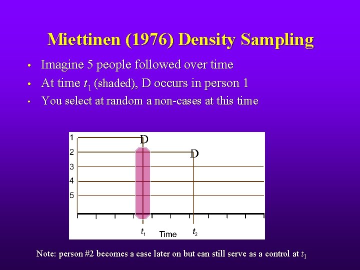
Miettinen (1976) Density Sampling • Imagine 5 people followed over time At time t 1 (shaded), D occurs in person 1 • You select at random a non-cases at this time • Note: person #2 becomes a case later on but can still serve as a control at t 1

How incidence density sampling works The ratio of exposed to non-exposed time in the controls estimates the ratio of exposed to nonexposed controls in the population (see EKS for details)

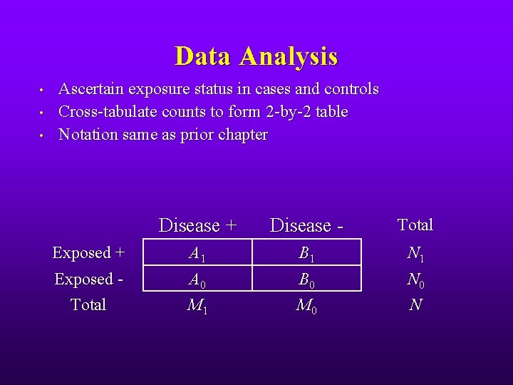
Data Analysis • • • Ascertain exposure status in cases and controls Cross-tabulate counts to form 2 -by-2 table Notation same as prior chapter Exposed + Exposed Total Disease + Disease - Total A 1 A 0 M 1 B 0 M 0 N 1 N 0 N

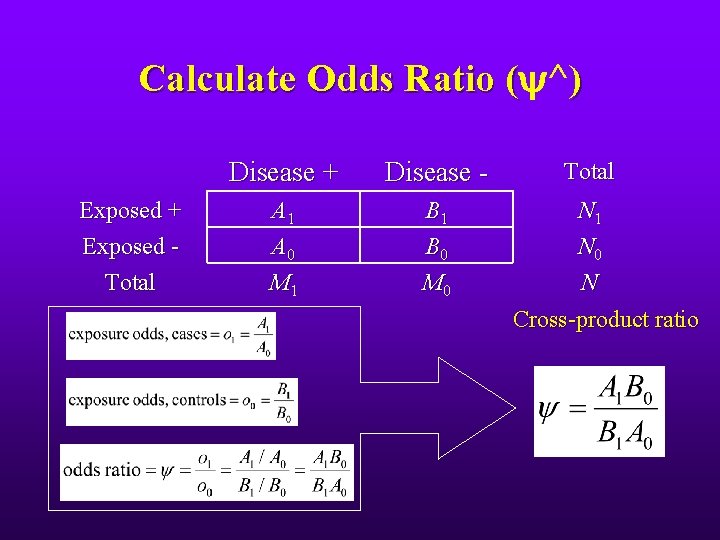
Calculate Odds Ratio ( ^) Exposed + Exposed Total Disease + Disease - Total A 1 A 0 M 1 B 0 M 0 N 1 N 0 N Cross-product ratio

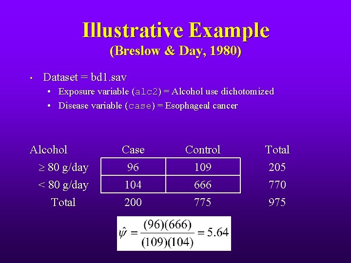
Illustrative Example (Breslow & Day, 1980) • Dataset = bd 1. sav • Exposure variable (alc 2) = Alcohol use dichotomized • Disease variable (case) = Esophageal cancer Alcohol 80 g/day < 80 g/day Total Case 96 104 200 Control 109 666 775 Total 205 770 975

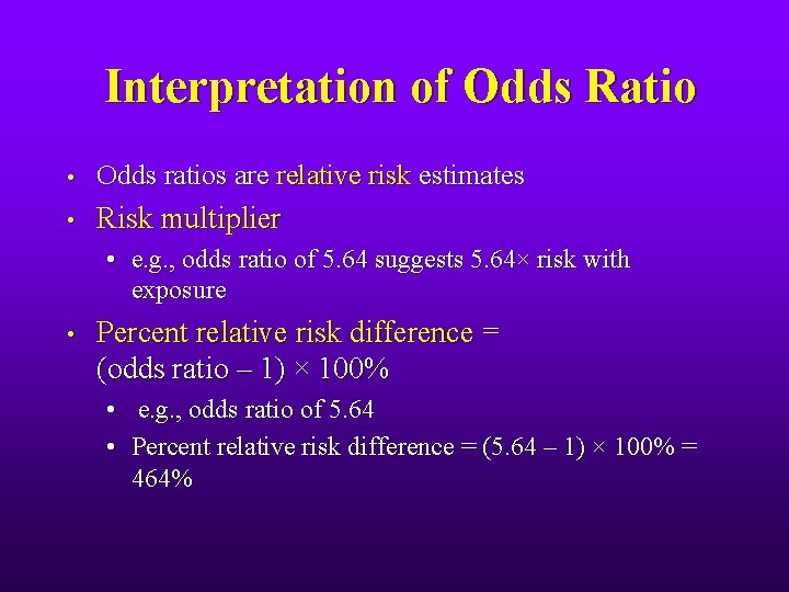
Interpretation of Odds Ratio • Odds ratios are relative risk estimates • Risk multiplier • e. g. , odds ratio of 5. 64 suggests 5. 64× risk with exposure • Percent relative risk difference = (odds ratio – 1) × 100% • e. g. , odds ratio of 5. 64 • Percent relative risk difference = (5. 64 – 1) × 100% = 464%

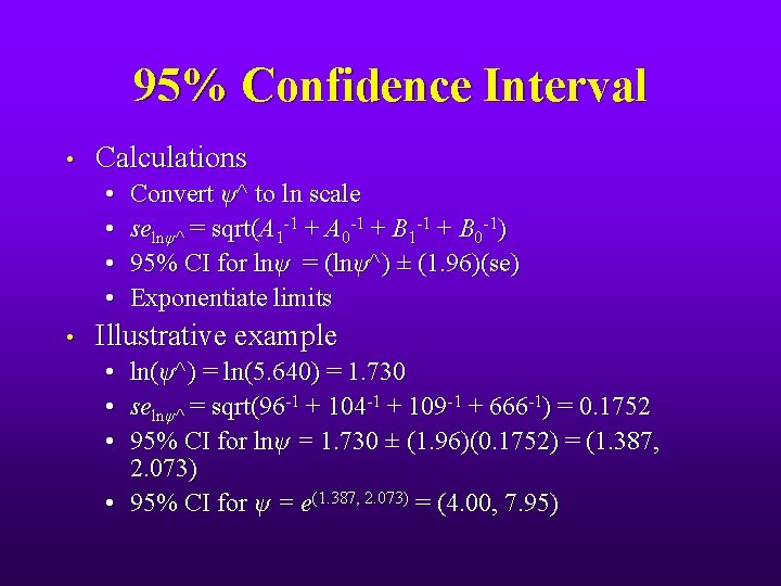
95% Confidence Interval • Calculations • • • Convert ψ^ to ln scale selnψ^ = sqrt(A 1 -1 + A 0 -1 + B 1 -1 + B 0 -1) 95% CI for lnψ = (lnψ^) ± (1. 96)(se) Exponentiate limits Illustrative example • ln(ψ^) = ln(5. 640) = 1. 730 • selnψ^ = sqrt(96 -1 + 104 -1 + 109 -1 + 666 -1) = 0. 1752 • 95% CI for lnψ = 1. 730 ± (1. 96)(0. 1752) = (1. 387, 2. 073) • 95% CI for ψ = e(1. 387, 2. 073) = (4. 00, 7. 95)

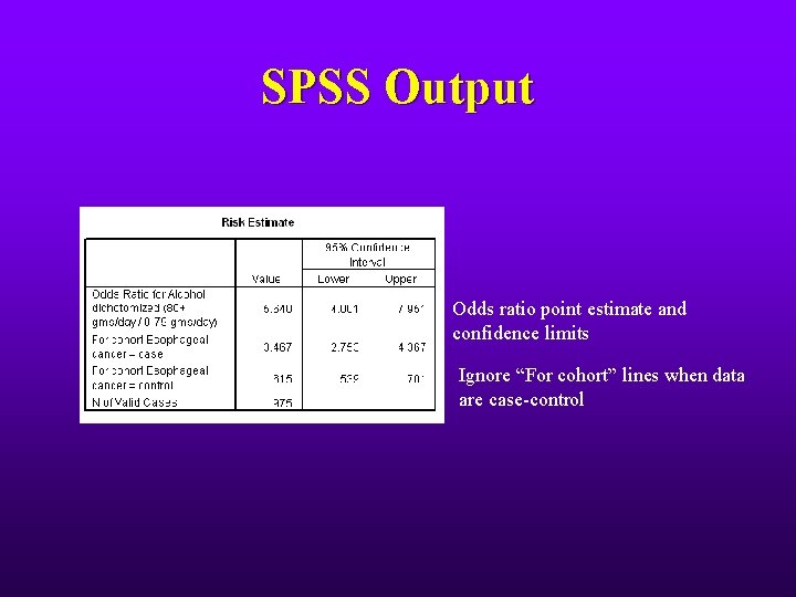
SPSS Output Odds ratio point estimate and confidence limits Ignore “For cohort” lines when data are case-control

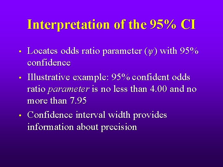
Interpretation of the 95% CI • • • Locates odds ratio parameter (ψ) with 95% confidence Illustrative example: 95% confident odds ratio parameter is no less than 4. 00 and no more than 7. 95 Confidence interval width provides information about precision

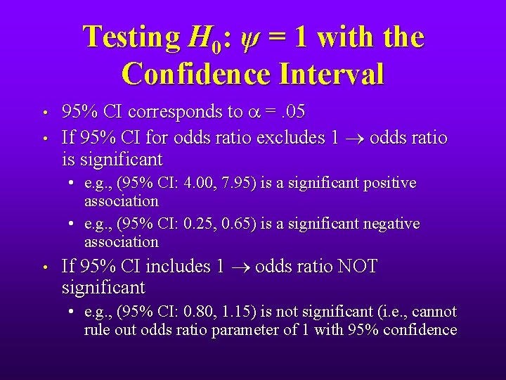
Testing H 0: ψ = 1 with the Confidence Interval • • 95% CI corresponds to a =. 05 If 95% CI for odds ratio excludes 1 odds ratio is significant • e. g. , (95% CI: 4. 00, 7. 95) is a significant positive association • e. g. , (95% CI: 0. 25, 0. 65) is a significant negative association • If 95% CI includes 1 odds ratio NOT significant • e. g. , (95% CI: 0. 80, 1. 15) is not significant (i. e. , cannot rule out odds ratio parameter of 1 with 95% confidence

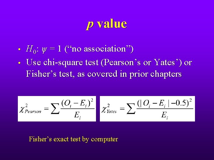
p value • • H 0: ψ = 1 (“no association”) Use chi-square test (Pearson’s or Yates’) or Fisher’s test, as covered in prior chapters Fisher’s exact test by computer

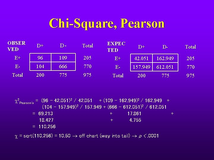
Chi-Square, Pearson OBSER VED D+ D- Total EXPEC TED D+ D- Total E+ 96 109 205 E+ 42. 051 162. 949 205 E- 104 666 770 E- 157. 949 612. 051 770 Total 200 775 975 c 2 Pearson's = (96 - 42. 051)2 / 42. 051 + (109 – 162. 949)2 / 162. 949 + (104 - 157. 949)2 / 157. 949 + (666 – 612. 051)2 / 612. 051 = 69. 213 + 17. 861 + 18. 427 + 4. 755 = 110. 256 c = sqrt(110. 256) = 10. 50 off chart (way into tail) p <. 0001

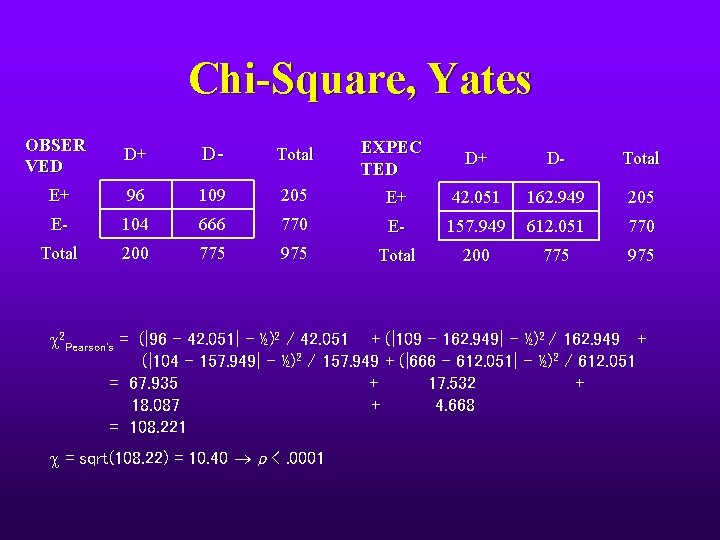
Chi-Square, Yates OBSER VED D+ D- Total EXPEC TED D+ D- Total E+ 96 109 205 E+ 42. 051 162. 949 205 E- 104 666 770 E- 157. 949 612. 051 770 Total 200 775 975 c 2 Pearson's = (|96 - 42. 051| - ½)2 / 42. 051 + (|109 – 162. 949| - ½)2 / 162. 949 + (|104 - 157. 949| - ½)2 / 157. 949 + (|666 – 612. 051| - ½)2 / 612. 051 = 67. 935 + 17. 532 + 18. 087 + 4. 668 = 108. 221 c = sqrt(108. 22) = 10. 40 p <. 0001

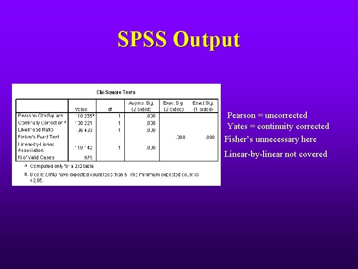
SPSS Output Pearson = uncorrected Yates = continuity corrected Fisher’s unnecessary here Linear-by-linear not covered

Interpreting the p value • • "If the null hypothesis were correct, the probability of observing the data is p“ e. g. , p =. 000 suggests association is unlikely due to chance (we can be confident in rejecting H 0)

Validity! • Before you get too carried away with the odds ratio (or any other statistic), remember they assume validity • No info bias (exposure and disease accurately classified) • No selection bias (cases and controls are fair reflection of population analogues) • No confounding

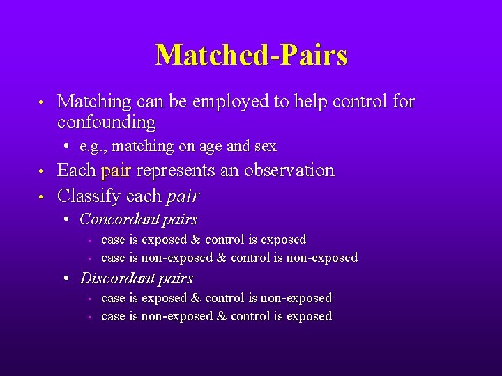
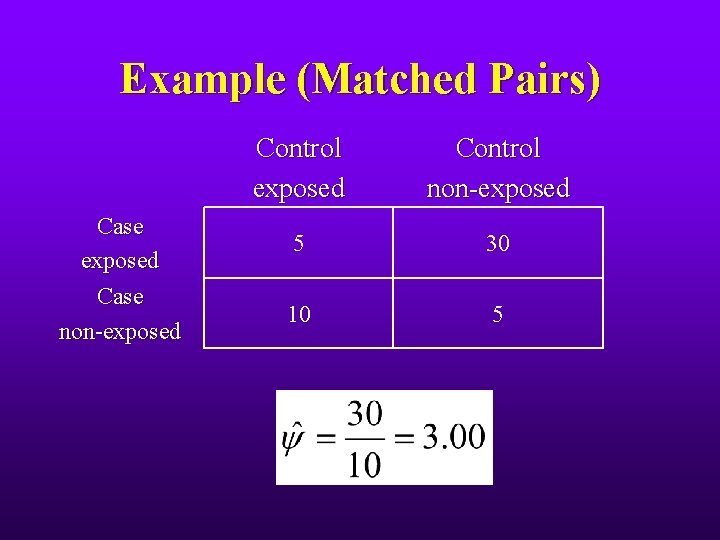
Matched-Pairs • Matching can be employed to help control for confounding • e. g. , matching on age and sex • • Each pair represents an observation Classify each pair • Concordant pairs • • case is exposed & control is exposed case is non-exposed & control is non-exposed • Discordant pairs • • case is exposed & control is non-exposed case is non-exposed & control is exposed

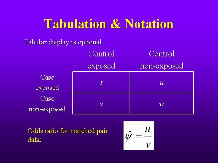
Tabulation & Notation Tabular display is optional Case exposed Case non-exposed Control non-exposed t u v w Odds ratio for matched pair data:

Example (Matched Pairs) Case exposed Case non-exposed Control non-exposed 5 30 10 5

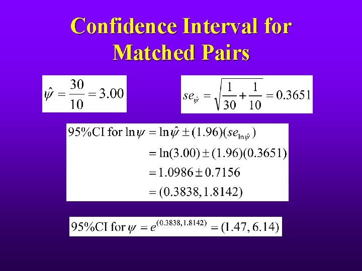
Confidence Interval for Matched Pairs

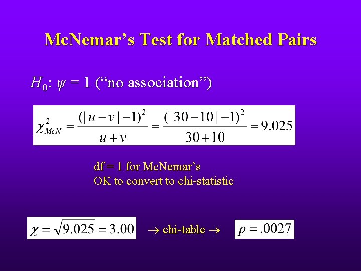
Mc. Nemar’s Test for Matched Pairs H 0: ψ = 1 (“no association”) df = 1 for Mc. Nemar’s OK to convert to chi-statistic chi-table