16 November 2016 st 1 Level Analysis Design

16 November 2016 st 1 Level Analysis Design Matrix, Contrasts and Inference, GLM Benjamin Chew and Rani Moran

Overview • Introduction • GLM • Design Matrix • Contrasts • Inference • Methodology

Our data Subject A Session 1 Volume Slice Voxel … … … Session 2 … Subject B … … …

Our data Subject A Session 1 Volume Slice Session 2 … Subject B … … … 1 st level analysis: within-subject analysis Voxel … analysing the time course of the f. MRI signal for every single subject separately

Our data Subject A Session 1 Volume Slice Voxel … … … Session 2 … Subject B … … … 2 nd level analysis: group level analysis

What are we looking at? • Our data is a time-series capturing changes in blood oxygenation (f. MRI signal intensities) in each voxel, tracked over the time of our experiment

Dealing with this data statistically • Mass univariate approach: using the same statistical analysis on every single voxel We are looking at the relationship between: • Y = dependent variable (BOLD signal) • X = regressor (experimental manipulation) • Null hypothesis: our experimental manipulation has no effect on Y • Our results are SPMs (Statistical Parametric Maps)

The General Linear Model observed data f. MRI time course in a particular voxel Adjust for the arbitrary units of the observed data (Y) regressor parameter component of our model which explains the observed data to some degree defines the contribution of X to the value of Y; it can be viewed as the slope of our regression line error (noise) the proportion of the variance in our data Y which is not explained by X

Mass univariate approach Matrix of BOLD signals Regressors

What is the Design Matrix?

Regressor Observation 1 Constant Modelling the condition: Modelling the constant:

The problem with our data

The problem with our data We know that a stimulus looking like this (Delta Function): will elicit a BOLD signal change like this: WE NEED TO ADJUST OUR MODEL FOR THIS!

HRF convolution Hemodynamic response function (HRF): Scaling Additivity Linear time-invariant (LTI) system: u(t) hrf(t) Convolution operator: x(t) Shift invariance Boynton et al, Neuro. Image, 2012.

Problem 1: BOLD response Solution: Convolution model

Convolution model of the BOLD response Convolve stimulus function with a canonical hemodynamic response function (HRF): HRF

The problem with our data • We have collected noisy data! • The signal we are interested in is relatively weak • The data has a complicated temporal and spatial noise structure

The problem with our data • Many types of noise in our data • E. g. head movement, physiological noise like heart beat/breathing or any non -modelled neural activity, scanner physics, susceptibility artefacts/dropout, … • The noise is not identically distributed or independent, but may affect some frequencies more than others • Much of this can be avoided by good quality acquisition, and by preprocessing • However, some of it may remain and has to be dealt with during analysis

Dealing with noise • Include nuisance regressors, e. g. for motion • High-pass filter to filter out low frequencies • We assume that most of the lower frequencies in our signal are due to noise, e. g. signal drift, so okay to exclude them • SPM default: 128 s

Our model • Our design matrix includes all available knowledge about experimentally controlled factors and potential confounds that may affect our data

Overview • Introduction • Design Matrix • GLM • Contrast • Inference • Methodology

Inference • After fitting the GLM we use the estimated parameters to determine whethere is significant activation present in the voxel • Inference is based on the fact that: • V accounts for temporal noise correlations • Use t and F procedures to perform tests on effects of interest

Hypothesis Testing To test a hypothesis, we construct “test statistics” • Null Hypothesis H 0 Typically what we want to reject (no effect) The Alternative Hypothesis HA expresses outcome of interest • Test Statistic T The test statistic summarises evidence about H 0 Typically, test statistic is small in magnitude when the hypothesis H 0 is true and large when false We need to know the distribution of T under the null hypothesis Null Distribution of T

Hypothesis Testing u • Significance level α: Acceptable false positive rate α. threshold uα Threshold uα controls the false positive rate Null Distribution of T • Conclusion about the hypothesis: We reject the null hypothesis in favour of the alternative hypothesis if t > uα • p-value: A p-value summarises evidence against H 0 This is the chance of observing value more extreme than t under the null hypothesis t p-value Null Distribution of T

Contrasts • It is often of interest to see whether a linear combination of the parameters are significant • The term c. Tβ specifies a linear combination of the estimated parameters, i. e. • Here c is called a contrast vector

Contrasts [1 10 -1 0 00 00 00 ]] [0

Example • Event-related experiment with two types of stimuli.

T-contrast • One-dimensional and directional • eg c. T = [ 1 0 0 0. . . ] tests β 1 > 0, against the null hypothesis H 0: β 1=0 • Equivalent to a one-tailed / unilateral t-test • Function: • Assess the effect of one parameter (c. T = [1 0 0 0]) OR • Compare specific combinations of parameters (c. T = [-1 1 0 0])

T-test • To test • use the t-statistic: T= contrast of estimated parameters variance estimate • Under H 0, T is approximately t(ν) with:

T-test summary • T-test is a simple signal-to-noise ratio measures • H 0: CT β=0 vs H 1: CT β>0 Y = X 1 * β 1 + X 2 * β 2 + β 3 + ε • “One” linear hypothesis testing • We can’t test both β 1=0 and β 2=0 at a same time • What if we have many interrelated experimental conditions, e. g. factorial design? • How can we test multiple linear hypothesis?

Multiple Contrasts • We often want to make simultaneous tests of several contrasts at once • Now c is a contrast matrix • Assume • Then

F-contrast • Multi-dimensional and non-directional • Tests whether at least one β is different from 0, against the null hypothesis H 0: β 1=β 2=β 3=0 • Equivalent to an ANOVA • Function: • Test multiple linear hypotheses, main effects, and interaction • But does NOT tell you which parameter is driving the effect nor the direction of the difference (F-contrast of β 1 -β 2 is the same thing as F-contrast of β 2 -β 1)

F-test - multidimensional contrasts – SPM{F} • Tests multiple linear hypotheses: H 0: True model is X 0 X 1 (b 4 -9) H 0: b 4 = b 5 =. . . = b 9 = 0 X 0 c. T = test H 0 : c. Tb = 0 ? 0001000001000001000 000000100 000000010 00001 SPM{F 6, 322} Full model? Reduced model?

F-test - the extra-sum-of-squares principle • Model comparison: Null Hypothesis H 0: True model is X 0 (reduced model) X 0 X 1 RSS Full model ? Test statistic: ratio of explained variability and unexplained variability (error) RSS 0 or Reduced model? 1 = rank(X) – rank(X 0) 2 = N – rank(X)

F-test summary • The F-test evaluates whether any combination of contrasts explains a significant amount of variability in the measured data • H 0: C β=0 vs H 1: C β≠ 0 • More flexible than T-test • F-test can tell the existence of significant contrasts. It does not tell which contrast drives the significant effect or what is the direction of the effect. • For a single contrast, F will implement a two sided T-test

Statistical Images • For each voxel a hypothesis test is performed. The statistic corresponding to that test is used to create a statistical image over all voxels.

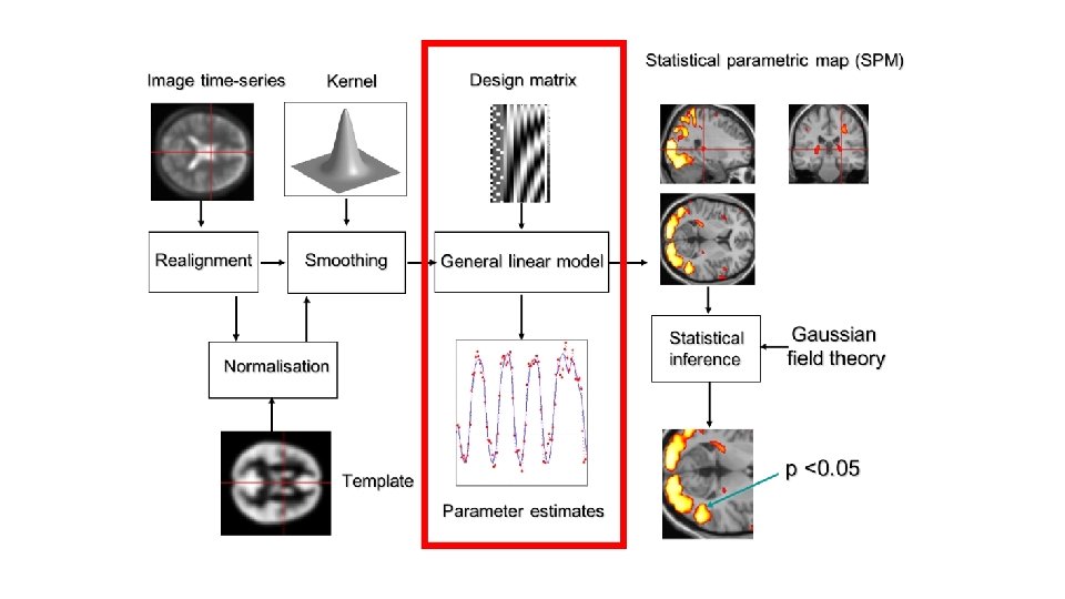
SPM Practical • Specify model: choose data files and set up design matrix • Estimate parameters using the GLM (either in the ‘traditional’ way or with Bayseian approaches) for every single voxel • Test hypotheses using contrast vectors. This produces a Statistical Parametric Map (or Posterior Probability Map in Bayesian models) • Interpretation

SPM Practical Brief Example: • 2 x 2 Factorial Design • Factor 1: Fame • Factor 2: Repetition • TE: 40 ms • TR: 2 s • 24 descending slices, 3 mm thick, 1. 5 mm gap

SPM Practical Simple example: • • • 2 conditions: listening to auditory stimuli, rest Blocks alternated between listening and rest Each acquisition consisted of 64 slices (3 x 3 mm 3 voxels) Acquisition took 6 s Scan repetition time (TR): 7 s (see SPM 12 Manual: Auditory f. MRI data)

SPECIFY st 1 LEVEL • After the pre-processing steps: Model specification • Press SPECIFY 1 ST LEVEL

SPECIFY st 1 LEVEL • In the batch editor, highlight “Directory” and select the location in which you want to save your results

SPECIFY st 1 LEVEL • Open “Timing Parameters”

SPECIFY st 1 LEVEL • Open “Timing Parameters” • Highlight “Units for Design” and select “Scans” (rather than “Seconds”) • Highlight “Interscan Interval” and enter your TR in seconds, e. g. 7

SPECIFY st 1 LEVEL • Highlight “Data and Design” and select “New Subject/Session” • Open the newly created “Subject/Session” option • Highlight “Scans” and select the smoothed, normalised functional images, e. g. swf. M 00*_00*. img

SPECIFY st 1 LEVEL • Highlight “Condition” and select “New Condition • Open the newly created “Condition” option • Highlight “Name” and enter the condition’s name, e. g. “Listening”

SPECIFY st 1 LEVEL • Highlight “Condition” and select “New Condition • Open the newly created “Condition” option • Highlight “Name” and enter the condition’s name, e. g. “Listening” • Highlight “Onsets” and enter the onset times of your condition, e. g. “ 6: 12: 84”

SPECIFY st 1 LEVEL • Highlight “Condition” and select “New Condition • Open the newly created “Condition” option • Highlight “Name” and enter the condition’s name, e. g. “Listening” • Highlight “Onsets” and enter the onset times of your condition, e. g. “ 6: 12: 84” • Highlight “Durations” and enter the duration of your condition in seconds, e. g. “ 6” • Save the batch as specify. mat • Press the RUN button

SPECIFY st 1 LEVEL • SPM will write an SPM. mat file to your directory • SPM will also plot the design matrix in the Graphics window • You can use the REVIEW button to check your model specification

ESTIMATE • After model specification: parameter estimation • Press the ESTIMATE button

ESTIMATE • Highlight the “Select SPM. mat” option and select the SPM. mat file you have saved earlier • Save the batch as estimate. mat • Press the RUN button • SPM will create a number of files in the selected directory, including a new version of the SPM. mat file

RESULTS • After parameter estimation: hypothesis testing • Press the RESULTS button

RESULTS • After parameter estimation: hypothesis testing • Press the RESULTS button • Select the SPM. mat file created by estimation

RESULTS • Select “Define new contrast” List of contrasts Surfable design matrix

RESULTS Select type of contrast • Select “Define new contrast” • Name your contrast, e. g. “Listening > Rest” • Select type of contrast: “t-contrast” or “F-contrast” • Use a numerical code to define your contrast, e. g. “[1 0]” Code your contrast

RESULTS • Select “Define new contrast” • Define a complementary contrast, e. g. “Rest > Listening”, and use the complementary code, e. g. “[-1 0]”

RESULTS • To view a contrast, select the name of the desired contrast, e. g. “Listening > Rest” • Press “Done”

RESULTS • Do you want to mask your results with a particular contrast? • By masking your results, you are only selecting those voxels which have been specified by the masking contrast (not applicable in our example) • In this case, select “none”

RESULTS • How do you want to set your statistical thresholds? • Select “FWE” • A family-wise error is a false positive anywhere in our SPM. This thresholding option uses “FWE-corrected” p-values

RESULTS • How do you want to set your statistical thresholds? • Select “FWE” • A family-wise error is a false positive anywhere in our SPM. This thresholding option uses “FWE-corrected” p-values • Select the default value of “ 0. 05”

RESULTS • What do you want your cluster extent threshold k to be? • Accept the default value, “ 0” • This will produce SPMs with clusters containing at least k (in our case, 0) voxels

RESULTS • SPM will show those voxels which reach our threshold in the “Listening > Rest” contrast in the Graphics window

RESULTS • SPM will also display a statistical table for our results

RESULTS • In SPM’s interactive window we can produce different statistical tables and visualisations of our data Statistical tables Visualisations

RESULTS • You can experiment with overlays to display your data

Take-home message The contrasts we can choose and the interpretation of results depend on our model specification, which in turn depends on our experimental design!

References • SPM 12 Manual: http: //www. fil. ion. ucl. ac. uk/spm/doc/manual. pdf (Ashburner et al. , 2015) • Introduction to Statistical Parametric Mapping: http: //www. fil. ion. ucl. ac. uk/spm/doc/intro/ (Friston, 2003) • Human Brain Function 2 nd edition: http: //www. fil. ion. ucl. ac. uk/spm/doc/books/hbf 2/ (Ashburner, Friston, & Penny), especially The general linear model (Kiebel & Holmes), Analysis of f. MRI timeseries: Linear time-invariant models, event-related f. MRI and optimal experimental design (Rik Henson), and Contrasts and classical inference (Poline, Kherif & Penny) • http: //editthis. info/scnlab/Analysis • Principles of Analysis: http: //imaging. mrc-cbu. cam. ac. uk/imaging/Analysis. Principles (Rik Henson) • Example Data Set from http: //www. fil. ion. ucl. ac. uk/spm/data/auditory/ • Slides from previous Mf. D presentations, inc. Elliot Freeman, Hugo Spiers, Beatriz Calvo & Davina Bristow, Ramiro & Sinead, Rebecca Knight & Lorelei Howard, Clare Palmer & Misun Kim • Slides from coursera SPM course • Joe Devlin’s slides from f. MRI Analysis course 2013 -14 • http: //www. anc. ed. ac. uk/CFIS/projects/prosody/material/slice 8. jpg • https: //www. sciencenews. org/sites/default/files/11543 • http: //www. brainvoyager. com/bvqx/doc/Users. Guide/Statistical. Analysis/The. General. Linear. Model. html • Pernet, C. R. (2014). Misconceptions in the use of the General Linear Model applied to functional MRI: a tutorial for junior neuro-imagers. Frontiers in Neuroscience, 8, 1. • Guillaume Flandin SPM Course slides • Christophe Phillips Contrasts and statistical inference