16 4 Competitive Market Efficiency Pareto Efficient No

16. 4 Competitive Market Efficiency Pareto Efficient » No alternate allocation of inputs and goods makes one consumer better off without hurting another consumer If another allocation improves AT LEAST ONE CONSUMER (without making anyone else worse off), the first allocation was Pareto Inefficient. 1

16. 4 Competitive Market Efficiency Pareto Efficiency has three requirements: 1) Exchange Efficiency Ø Goods cannot be traded to make a consumer better off 2) Input Efficiency Ø Inputs cannot be rearranged to produce more goods 2

16. 4 Competitive Market Efficiency 3) Substitution Efficiency Ø Substituting one good for another will not make one consumer better off without harming another consumer 3

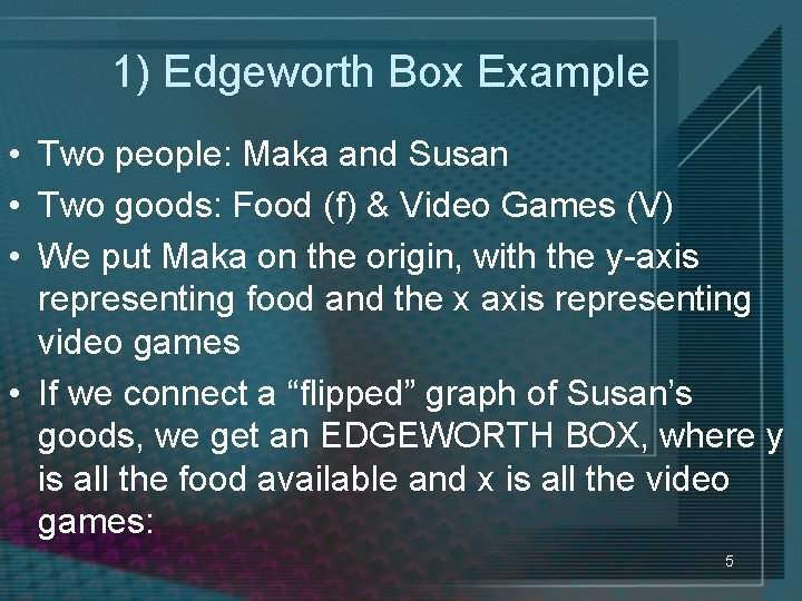
1) Exchange Efficiency Model Assumptions • Assumptions: – 2 people – 2 goods, each of fixed quantity ØThis allows us to construct an EDGEWORTH BOX – a graph showing all the possible allocations of goods in a twogood economy, given the total available supply of each good 4

1) Edgeworth Box Example • Two people: Maka and Susan • Two goods: Food (f) & Video Games (V) • We put Maka on the origin, with the y-axis representing food and the x axis representing video games • If we connect a “flipped” graph of Susan’s goods, we get an EDGEWORTH BOX, where y is all the food available and x is all the video games: 5

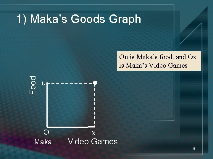
1) Maka’s Goods Graph Food Ou is Maka’s food, and Ox is Maka’s Video Games u O Maka x Video Games 6

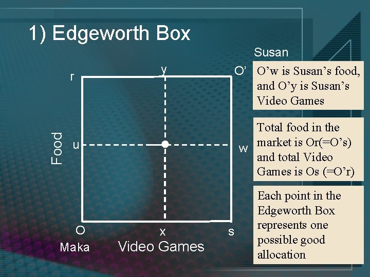
1) Edgeworth Box Susan Food r y O’ O’w is Susan’s food, and O’y is Susan’s Video Games Total food in the w market is Or(=O’s) and total Video Games is Os (=O’r) u O Maka x Video Games s Each point in the Edgeworth Box represents one possible good allocation 7

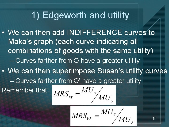
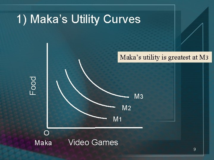
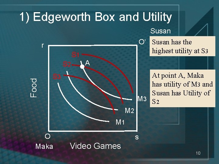
1) Edgeworth and utility • We can then add INDIFFERENCE curves to Maka’s graph (each curve indicating all combinations of goods with the same utility) – Curves farther from O have a greater utility • We can then superimpose Susan’s utility curves – Curves farther from O’ have a greater utility Remember that: 8

1) Maka’s Utility Curves Food Maka’s utility is greatest at M 3 M 2 M 1 O Maka Video Games 9

1) Edgeworth Box and Utility Susan O’ Susan has the highest utility at S 3 r S 1 Food S 2 A At point A, Maka has utility of M 3 and Susan has Utility of M 3 S 2 S 3 M 2 M 1 O Maka s Video Games 10

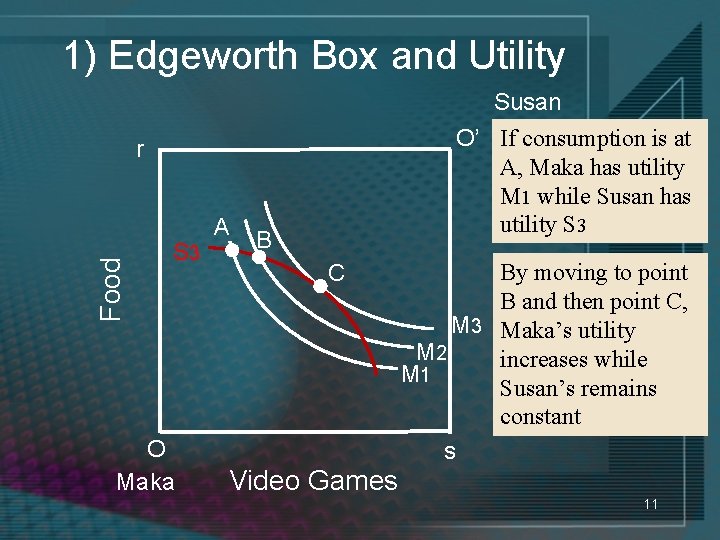
1) Edgeworth Box and Utility Susan O’ If consumption is at A, Maka has utility M 1 while Susan has utility S 3 Food r S 3 O Maka A B C By moving to point B and then point C, M 3 Maka’s utility M 2 increases while M 1 Susan’s remains constant s Video Games 11

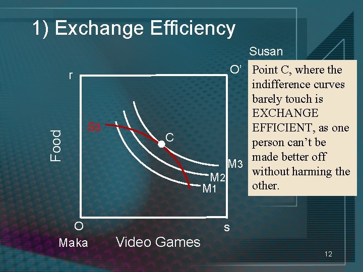
1) Exchange Efficiency Susan Food r S 3 O Maka C O’ Point C, where the indifference curves barely touch is EXCHANGE EFFICIENT, as one person can’t be made better off M 3 without harming the M 2 other. M 1 s Video Games 12

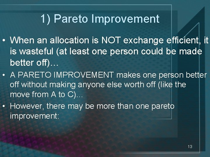
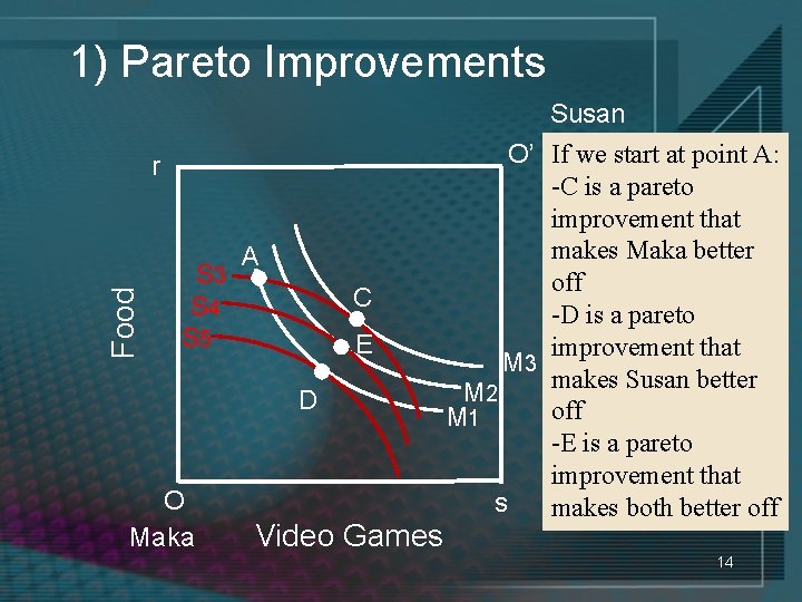
1) Pareto Improvement • When an allocation is NOT exchange efficient, it is wasteful (at least one person could be made better off)… • A PARETO IMPROVEMENT makes one person better off without making anyone else worth off (like the move from A to C)… • However, there may be more than one pareto improvement: 13

1) Pareto Improvements Susan Food r S 3 S 4 S 5 A C E D O Maka Video Games O’ If we start at point A: -C is a pareto improvement that makes Maka better off -D is a pareto improvement that M 3 makes Susan better M 2 off M 1 -E is a pareto improvement that s makes both better off 14

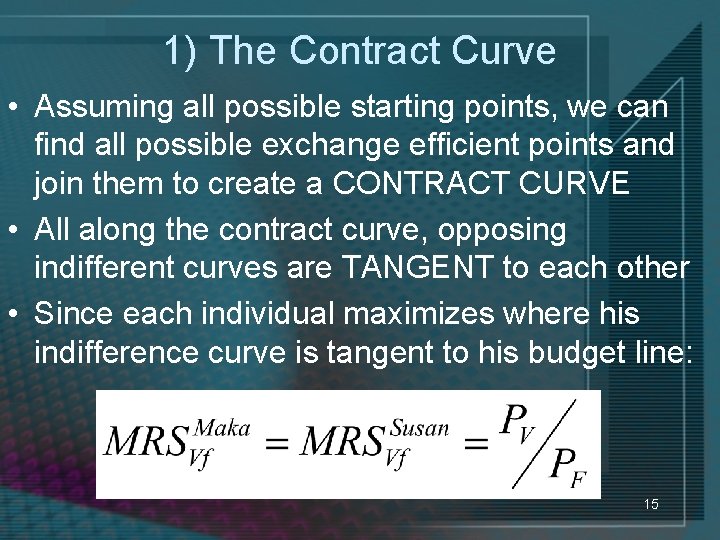
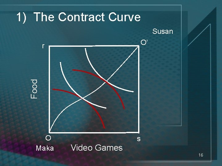
1) The Contract Curve • Assuming all possible starting points, we can find all possible exchange efficient points and join them to create a CONTRACT CURVE • All along the contract curve, opposing indifferent curves are TANGENT to each other • Since each individual maximizes where his indifference curve is tangent to his budget line: 15

1) The Contract Curve Susan O’ Food r O Maka s Video Games 16

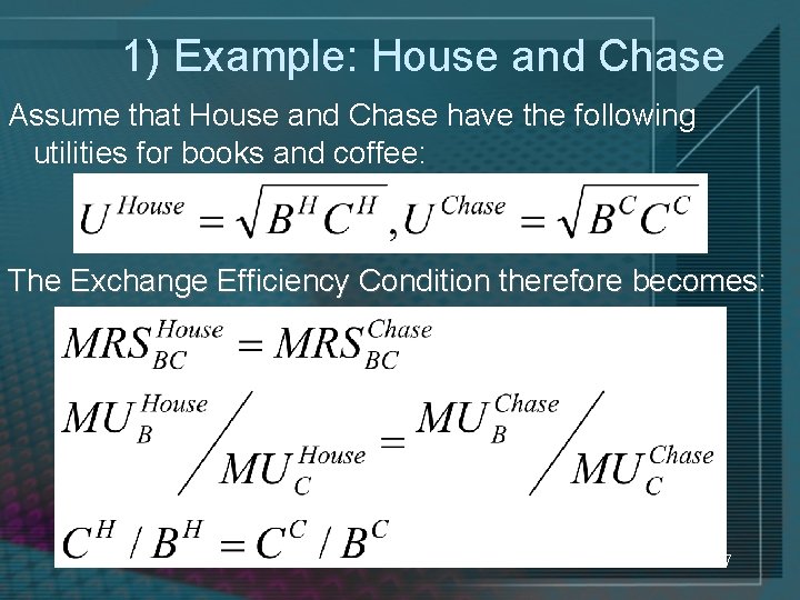
1) Example: House and Chase Assume that House and Chase have the following utilities for books and coffee: The Exchange Efficiency Condition therefore becomes: 17

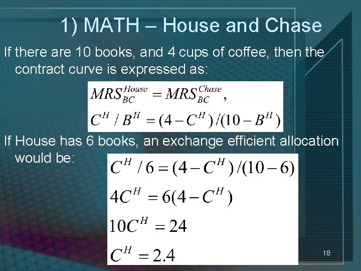
1) MATH – House and Chase If there are 10 books, and 4 cups of coffee, then the contract curve is expressed as: If House has 6 books, an exchange efficient allocation would be: 18

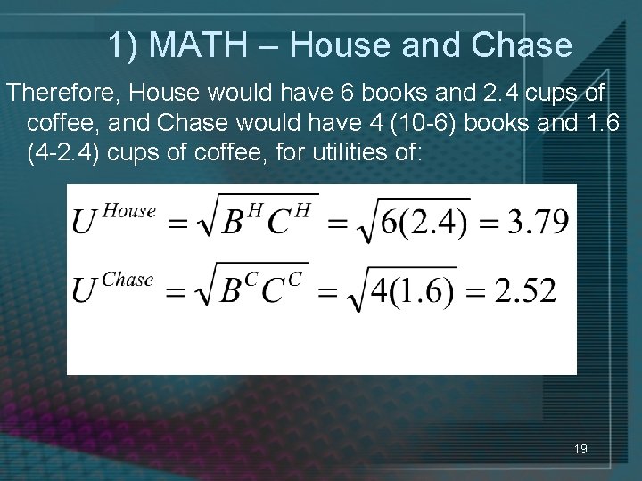
1) MATH – House and Chase Therefore, House would have 6 books and 2. 4 cups of coffee, and Chase would have 4 (10 -6) books and 1. 6 (4 -2. 4) cups of coffee, for utilities of: 19

2) Input Efficiency Model Assumptions • Assumptions: – 2 producers/firms – 2 inputs (Labor and Capital), each of fixed quantity ØThis lead to a EDGEWORTH BOX FOR INPUTS– a graph showing all the possible allocations of fixed quantities of labor and capital between two producers 20

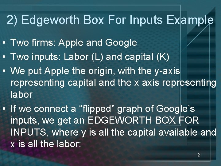
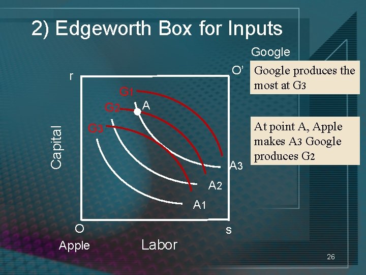
2) Edgeworth Box For Inputs Example • Two firms: Apple and Google • Two inputs: Labor (L) and capital (K) • We put Apple the origin, with the y-axis representing capital and the x axis representing labor • If we connect a “flipped” graph of Google’s inputs, we get an EDGEWORTH BOX FOR INPUTS, where y is all the capital available and x is all the labor: 21

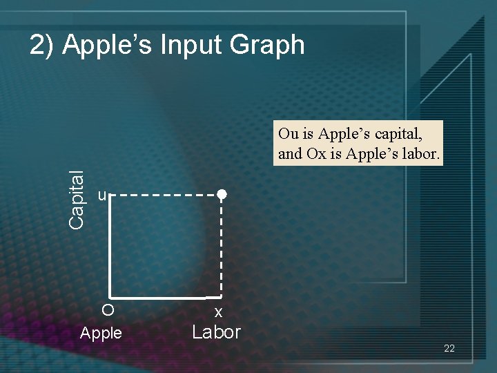
2) Apple’s Input Graph Capital Ou is Apple’s capital, and Ox is Apple’s labor. u O Apple x Labor 22

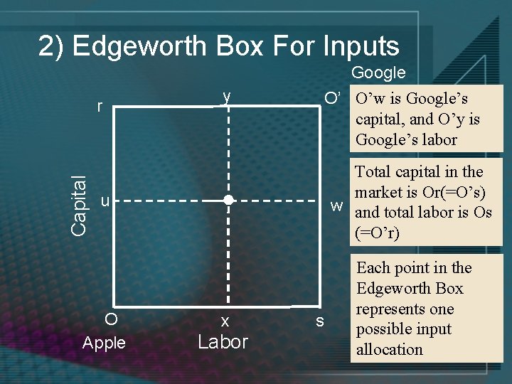
2) Edgeworth Box For Inputs Google Capital r y O’ O’w is Google’s capital, and O’y is Google’s labor Total capital in the market is Or(=O’s) w and total labor is Os (=O’r) u O Apple x Labor s Each point in the Edgeworth Box represents one possible input allocation 23

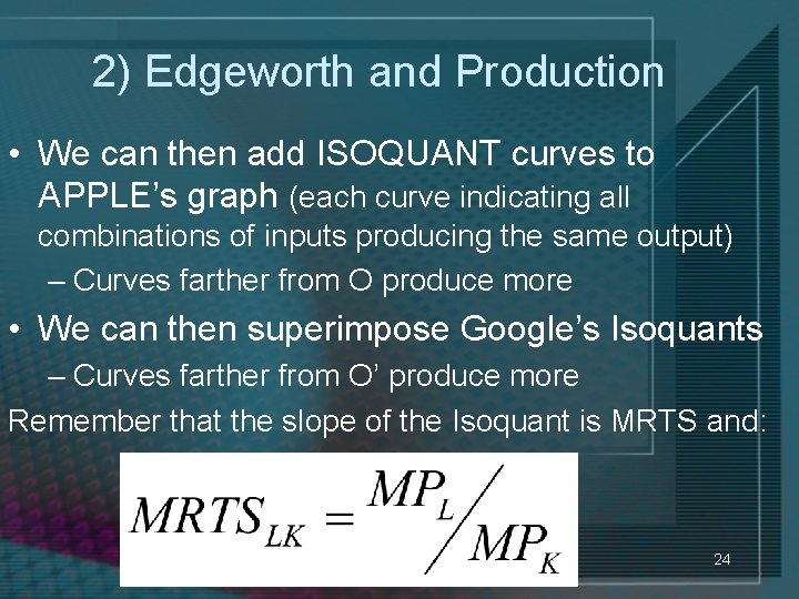
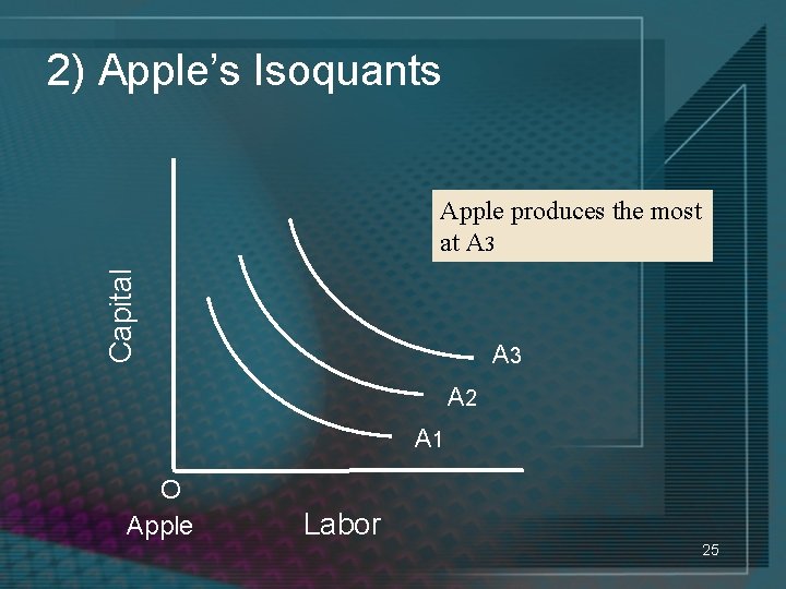
2) Edgeworth and Production • We can then add ISOQUANT curves to APPLE’s graph (each curve indicating all combinations of inputs producing the same output) – Curves farther from O produce more • We can then superimpose Google’s Isoquants – Curves farther from O’ produce more Remember that the slope of the Isoquant is MRTS and: 24

2) Apple’s Isoquants Capital Apple produces the most at A 3 A 2 A 1 O Apple Labor 25

2) Edgeworth Box for Inputs Google O’ Google produces the most at G 3 r G 1 Capital G 2 A G 3 At point A, Apple makes A 3 Google produces G 2 A 1 O Apple s Labor 26

2) Edgeworth Box and Utility Google O’ If production is at A, Apple produces A 1 while Google produces G 3 Capital r G 3 O Apple A B C By moving to point B and then point C, A 3 Apple produces A 2 more while A 1 Google’s production remains constant s Labor 27

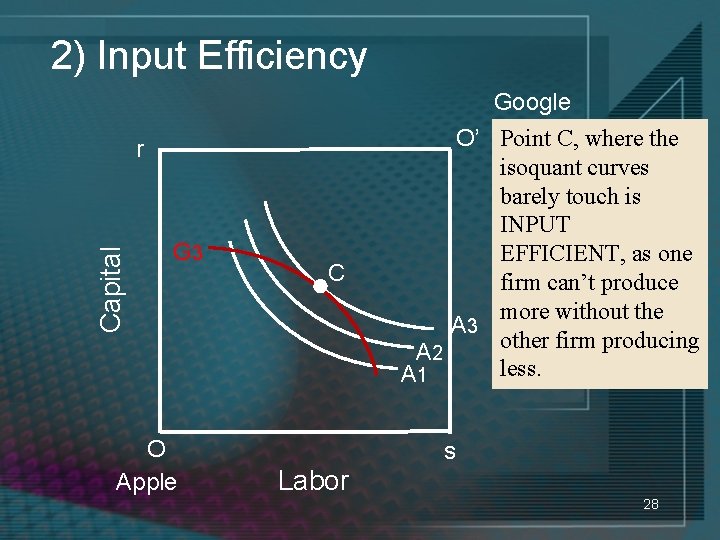
2) Input Efficiency Google Capital r G 3 O Apple C O’ Point C, where the isoquant curves barely touch is INPUT EFFICIENT, as one firm can’t produce more without the A 3 other firm producing A 2 less. A 1 s Labor 28

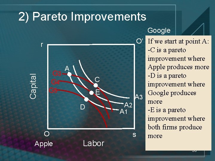
2) Pareto Improvement • When an input allocation is NOT input efficient, it is wasteful (at least one firm COULD produce more)… • A PARETO IMPROVEMENT allows one firm to produce more without reducing the output of the other firm(like the move from A to C) • However, there may be more than one pareto improvement: 29

2) Pareto Improvements Google Capital r G 3 G 4 G 5 A C E D O Apple Labor O’ If we start at point A: -C is a pareto improvement where Apple produces more -D is a pareto improvement where Google produces A 3 more A 2 -E is a pareto A 1 improvement where both firms produce s more 30

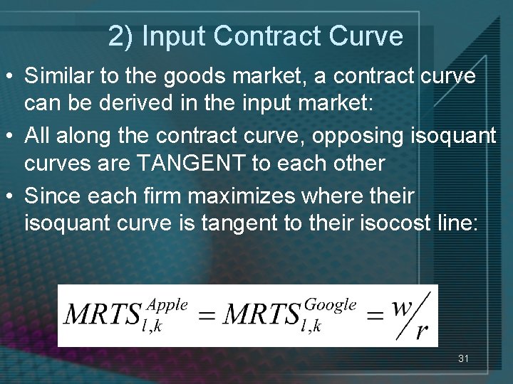
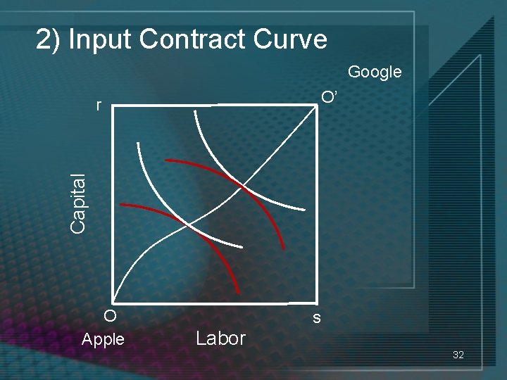
2) Input Contract Curve • Similar to the goods market, a contract curve can be derived in the input market: • All along the contract curve, opposing isoquant curves are TANGENT to each other • Since each firm maximizes where their isoquant curve is tangent to their isocost line: 31

2) Input Contract Curve Google O’ Capital r O Apple s Labor 32

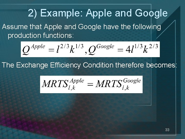
2) Example: Apple and Google Assume that Apple and Google have the following production functions: The Exchange Efficiency Condition therefore becomes: 33

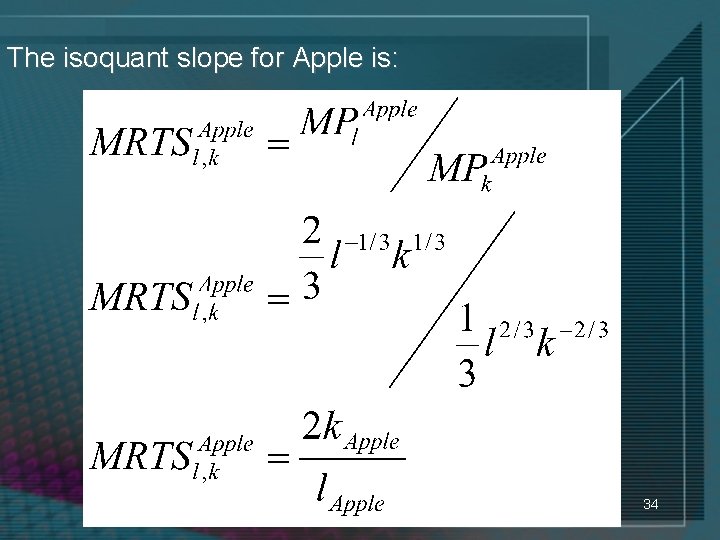
The isoquant slope for Apple is: 34

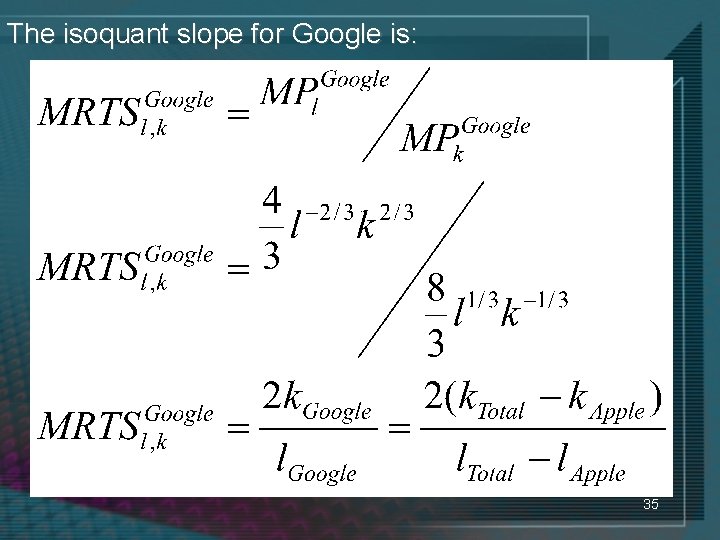
The isoquant slope for Google is: 35

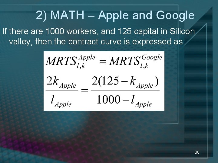
2) MATH – Apple and Google If there are 1000 workers, and 125 capital in Silicon valley, then the contract curve is expressed as: 36

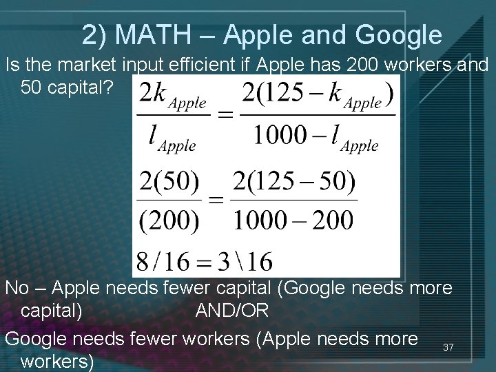
2) MATH – Apple and Google Is the market input efficient if Apple has 200 workers and 50 capital? No – Apple needs fewer capital (Google needs more capital) AND/OR Google needs fewer workers (Apple needs more 37 workers)

3) Substitution Efficiency • Substitution Efficiency can be analyzed using the PRODUCTION POSSIBILITIES CURVE/FRONTIER – The PPC shows all combinations of 2 goods that can be produced using available inputs – The slope of the PPC shows how much of one good must be SUBSTITUTED to produce more of the other good, or MARGINAL RATE OF TRANSFORMATION (x for y) (MRTxy) 38

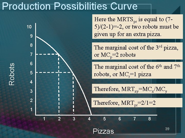
Production Possibilities Curve Here the MRTSpr is equal to (75)/(2 -1)=-2, or two robots must be given up for an extra pizza. 10 9 8 The marginal cost of the 3 rd pizza, or MCp=2 robots Robots 7 6 The marginal cost of the 6 th and 7 th robots, or MCr=1 pizza 5 4 Therefore, MRTxy=MCx/MCy 3 2 Therefore, MRTpr=2/1=2 1 1 2 3 4 5 Pizzas 6 7 8 39

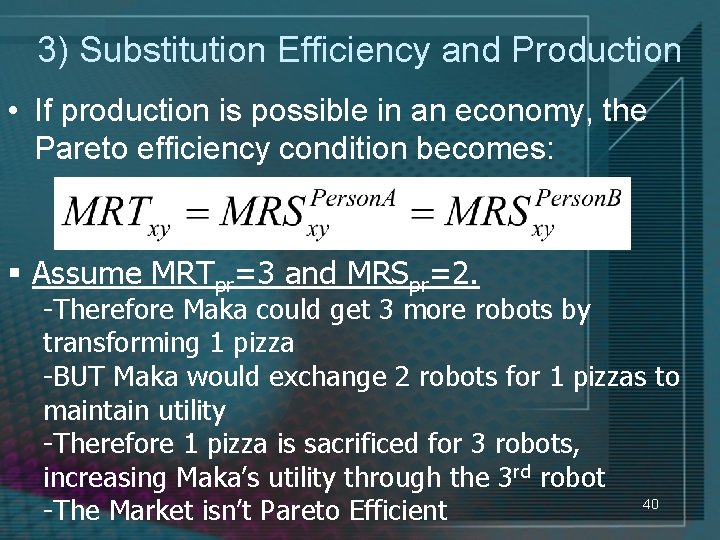
3) Substitution Efficiency and Production • If production is possible in an economy, the Pareto efficiency condition becomes: § Assume MRTpr=3 and MRSpr=2. -Therefore Maka could get 3 more robots by transforming 1 pizza -BUT Maka would exchange 2 robots for 1 pizzas to maintain utility -Therefore 1 pizza is sacrificed for 3 robots, increasing Maka’s utility through the 3 rd robot 40 -The Market isn’t Pareto Efficient

The First Fundamental Theorem Of Welfare Economics IF 1) All consumers and producers act as perfect competitors (no one has market power) and 2) A market exists for each and every commodity Then Resource allocation is Pareto Efficient 41

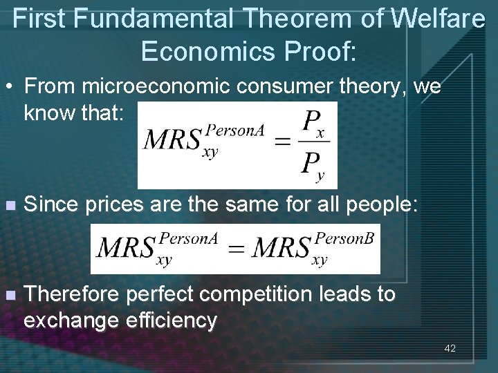
First Fundamental Theorem of Welfare Economics Proof: • From microeconomic consumer theory, we know that: n Since prices are the same for all people: n Therefore perfect competition leads to exchange efficiency 42

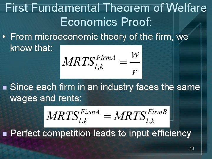
First Fundamental Theorem of Welfare Economics Proof: • From microeconomic theory of the firm, we know that: n Since each firm in an industry faces the same wages and rents: n Perfect competition leads to input efficiency 43

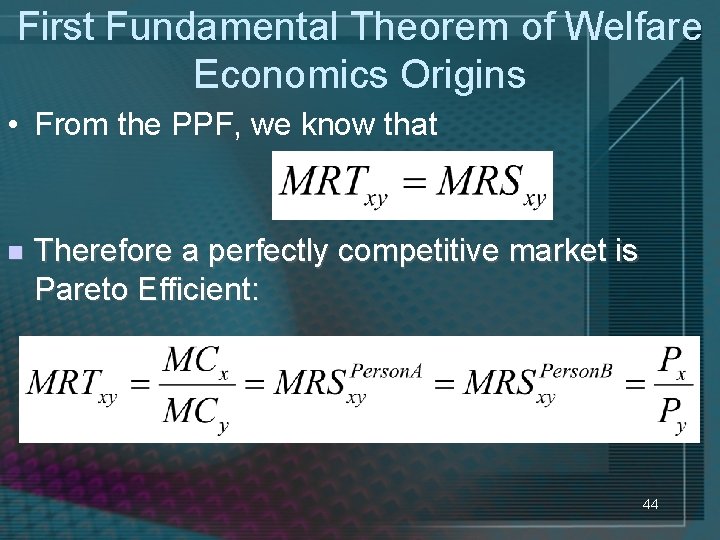
First Fundamental Theorem of Welfare Economics Origins • From the PPF, we know that n Therefore a perfectly competitive market is Pareto Efficient: 44

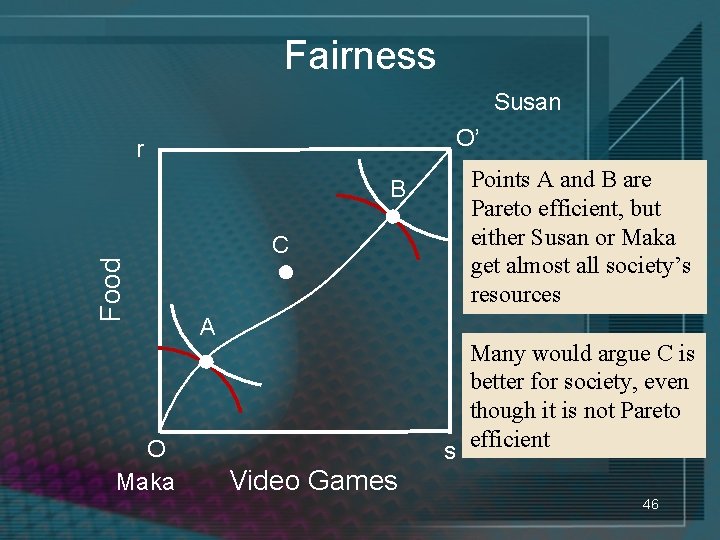
Efficiency≠Fairness • If Pareto Efficiency was the only concern, competitive markets automatically achieve it and there would be very little need for government: – Government would exist to protect property rights • Laws, Courts, and National Defense • But Pareto Efficiency doesn’t consider distribution. One person could get all society’s resources while everyone else starves. This 45 isn’t typically socially optimal.

Fairness Susan O’ r Food B O Maka C A Points A and B are Pareto efficient, but either Susan or Maka get almost all society’s resources Many would argue C is better for society, even though it is not Pareto s efficient Video Games 46

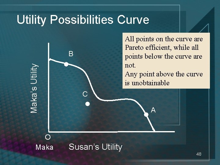
Fairness • For each utility level of one person, there is a maximum utility of the other • Graphing each utility against the other gives us the UTILITY POSSIBILITIES CURVE: 47

Utility Possibilities Curve All points on the curve are Pareto efficient, while all points below the curve are not. Any point above the curve is unobtainable Maka’s Utility B O Maka C A Susan’s Utility 48

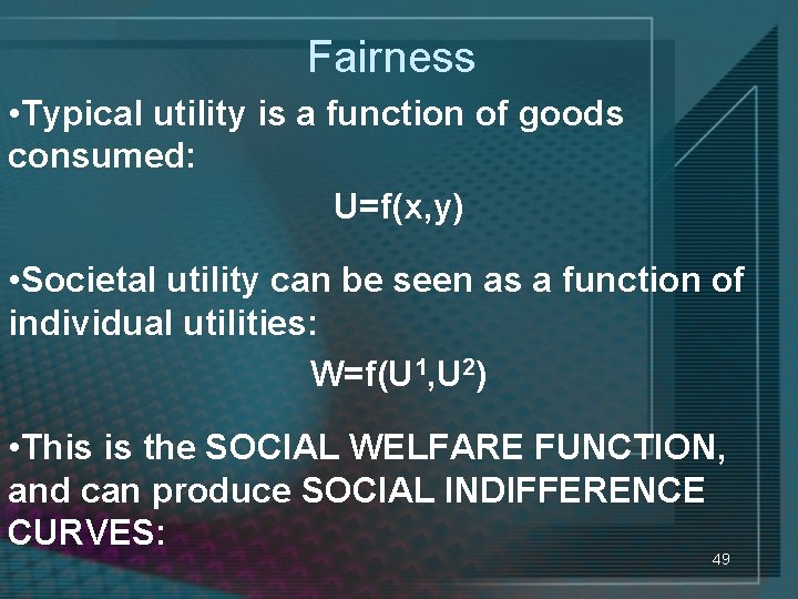
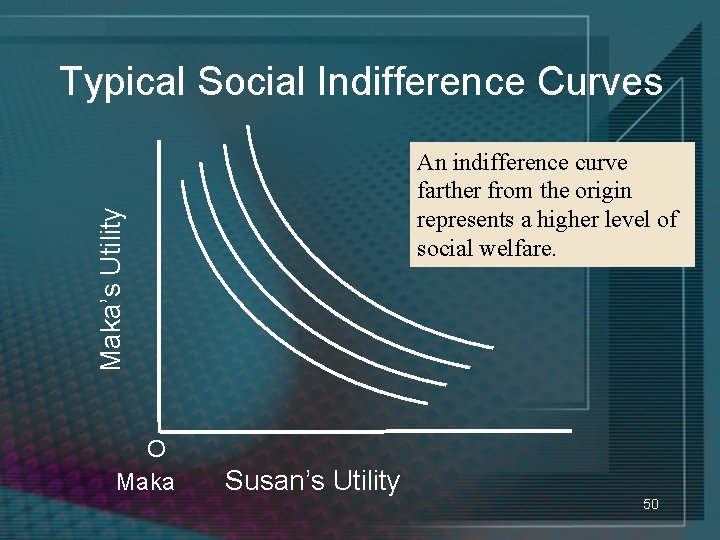
Fairness • Typical utility is a function of goods consumed: U=f(x, y) • Societal utility can be seen as a function of individual utilities: W=f(U 1, U 2) • This is the SOCIAL WELFARE FUNCTION, and can produce SOCIAL INDIFFERENCE CURVES: 49

Typical Social Indifference Curves Maka’s Utility An indifference curve farther from the origin represents a higher level of social welfare. O Maka Susan’s Utility 50

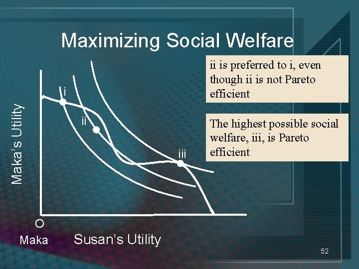
Fairness • If we superimpose social indifference curves on top of the utilities possibilities curve, we can find the Pareto efficient point that maximizes social welfare • This leads us to the SECOND FUNDAMENTAL THEOREM OF WELFARE ECONOMICS 51

Maximizing Social Welfare ii is preferred to i, even though ii is not Pareto efficient Maka’s Utility i O Maka ii iii The highest possible social welfare, iii, is Pareto efficient Susan’s Utility 52

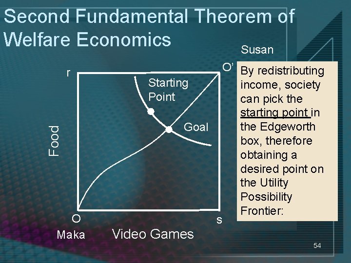
Second Fundamental Theorem of Welfare Economics The SECOND FUNDAMENTAL THEOREM OF WELFARE ECONOMICS states that: Society can attain any Pareto efficient allocation of resources by: 1) making a suitable assignments of original endowments, and then 2) letting people trade 53

Second Fundamental Theorem of Welfare Economics Susan Food r O Maka O’ By redistributing Starting income, society Point can pick the starting point in the Edgeworth Goal box, therefore obtaining a desired point on the Utility Possibility Frontier: s Video Games 54

Why Is Government so Big? 1) Government has to ensure property laws are protected. (1 st Theorem) 2) Government has to redistribute income to achieve equity. (2 nd Theorem) 3) Often the assumptions of the First Welfare Theorem do not hold (Econ 350) 55

Why Trade and Not Tax? Taxes and penalties punish income-enhancing behavior, encouraging people to work less. Subsidies and incentives give an incentive to stay in a negative state to keep receiving subsidies and incentives. Lump sum transfers have the least distortion, AND TRADE ALWAYS BENEFITS BOTH PARTIES… 56

16. 5 Gains From Free Trade • Trade ALWAYS makes society better off by increasing the productivity of scarce resources • The basis for the gains from specialization and trade is Comparative Advantage 57

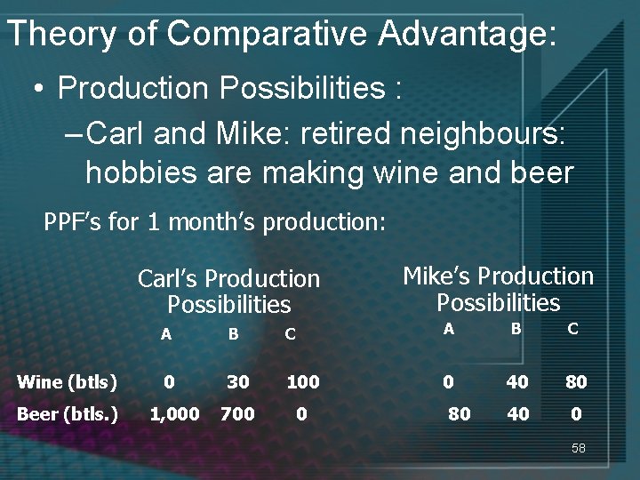
Theory of Comparative Advantage: • Production Possibilities : – Carl and Mike: retired neighbours: hobbies are making wine and beer PPF’s for 1 month’s production: Carl’s Production Possibilities Mike’s Production Possibilities A B C Wine (btls) 0 30 100 0 40 80 Beer (btls. ) 1, 000 700 0 80 40 0 58

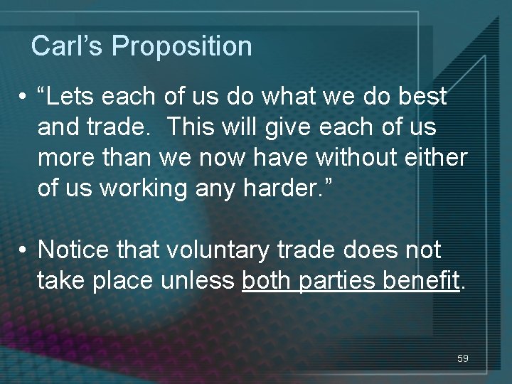
Carl’s Proposition • “Lets each of us do what we do best and trade. This will give each of us more than we now have without either of us working any harder. ” • Notice that voluntary trade does not take place unless both parties benefit. 59

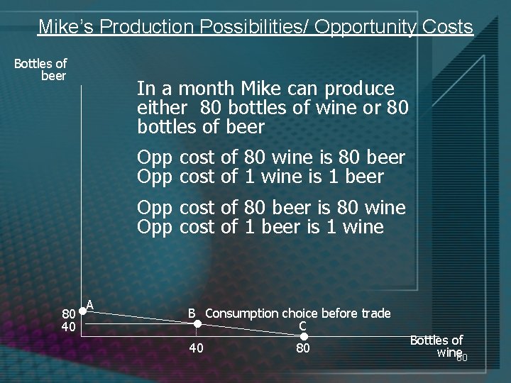
Mike’s Production Possibilities/ Opportunity Costs Bottles of beer In a month Mike can produce either 80 bottles of wine or 80 bottles of beer Opp cost of 80 wine is 80 beer Opp cost of 1 wine is 1 beer Opp cost of 80 beer is 80 wine Opp cost of 1 beer is 1 wine 80 40 • A B Consumption choice before trade C • 40 • 80 Bottles of wine 60

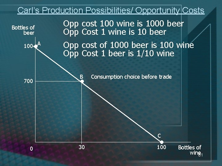
Carl’s Production Possibilities/ Opportunity Costs Bottles of beer • 100 A 700 Opp cost 100 wine is 1000 beer Opp Cost 1 wine is 10 beer Opp cost of 1000 beer is 100 wine Opp Cost 1 beer is 1/10 wine B • Consumption choice before trade C 0 30 • 100 Bottles of wine 61

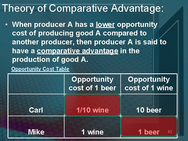
Theory of Comparative Advantage: • When producer A has a lower opportunity cost of producing good A compared to another producer, then producer A is said to have a comparative advantage in the production of good A. Opportunity Cost Table Opportunity cost of 1 beer Opportunity cost of 1 wine Carl 1/10 wine 10 beer Mike 1 wine 1 beer 62

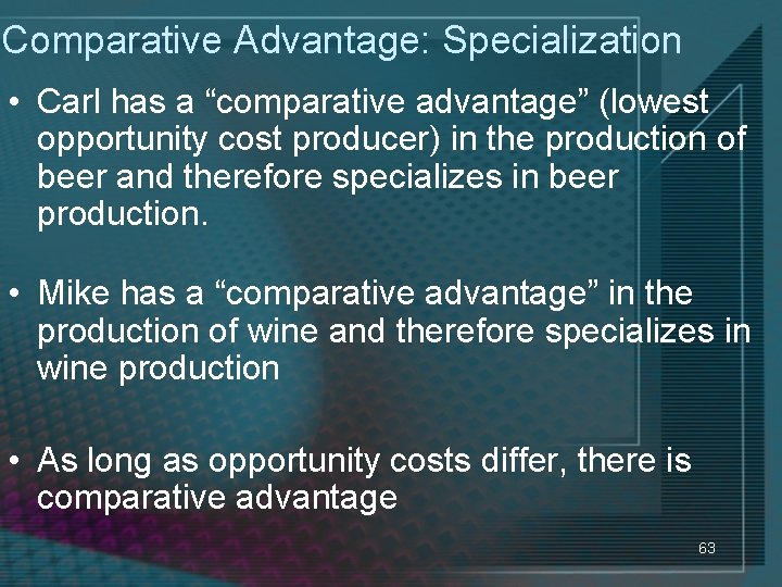
Comparative Advantage: Specialization • Carl has a “comparative advantage” (lowest opportunity cost producer) in the production of beer and therefore specializes in beer production. • Mike has a “comparative advantage” in the production of wine and therefore specializes in wine production • As long as opportunity costs differ, there is comparative advantage 63

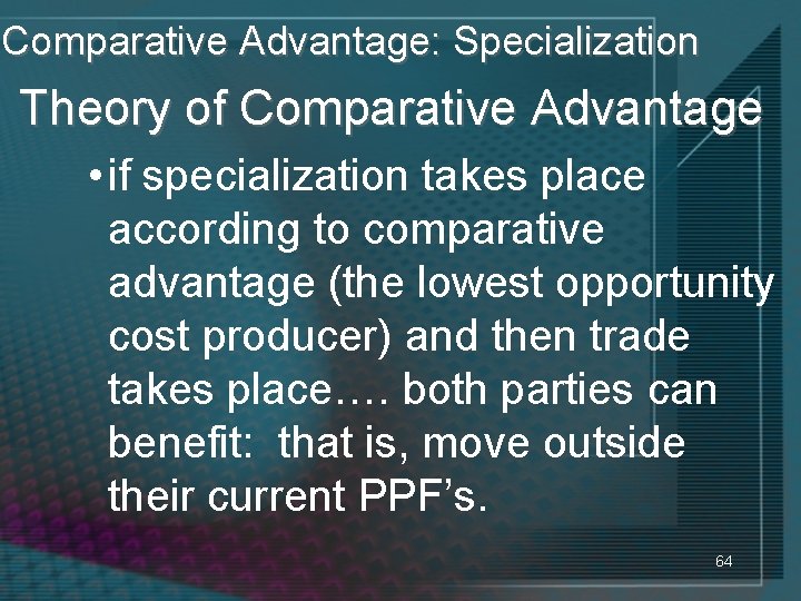
Comparative Advantage: Specialization Theory of Comparative Advantage • if specialization takes place according to comparative advantage (the lowest opportunity cost producer) and then trade takes place…. both parties can benefit: that is, move outside their current PPF’s. 64

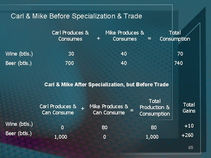
Carl & Mike Before Specialization & Trade Carl Produces & Consumes Mike Produces & + = Consumes Total Consumption Wine (btls. ) 30 40 70 Beer (btls. ) 700 40 740 Carl & Mike After Specialization, but Before Trade Carl Produces & + Mike Produces & = Can Consume Wine (btls. ) Beer (btls. ) 0 1, 000 80 0 Total Production & Consumption Total Gains 80 +10 1, 000 +260 65

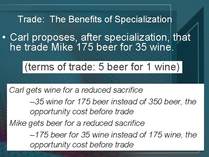
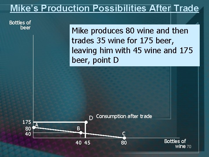
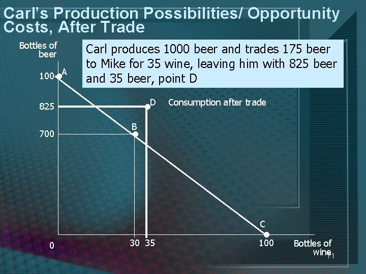
Trade: The Benefits of Specialization • Carl proposes, after specialization, that he trade Mike 175 beer for 35 wine. (terms of trade: 5 beer for 1 wine) Carl gets wine for a reduced sacrifice – 35 wine for 175 beer instead of 350 beer, the opportunity cost before trade Mike gets beer for a reduced sacrifice – 175 beer for 35 wine instead of 175 wine, the opportunity cost before trade 66

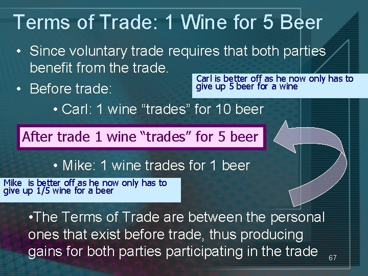
Terms of Trade: 1 Wine for 5 Beer • Since voluntary trade requires that both parties benefit from the trade. Carl is better off as he now only has to give up 5 beer for a wine • Before trade: • Carl: 1 wine “trades” for 10 beer After trade 1 wine “trades” for 5 beer • Mike: 1 wine trades for 1 beer Mike is better off as he now only has to give up 1/5 wine for a beer • The Terms of Trade are between the personal ones that exist before trade, thus producing gains for both parties participating in the trade 67

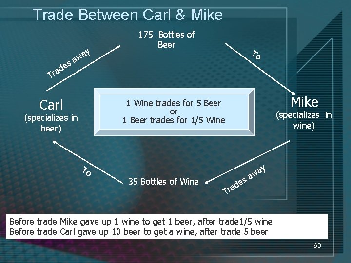
Trade Between Carl & Mike y wa a s 175 Bottles of Beer To e d a r T Carl Mike 1 Wine trades for 5 Beer or 1 Beer trades for 1/5 Wine (specializes in beer) To 35 Bottles of Wine (specializes in wine) s de y a w a Tra Before trade Mike gave up 1 wine to get 1 beer, after trade 1/5 wine Before trade Carl gave up 10 beer to get a wine, after trade 5 beer 68

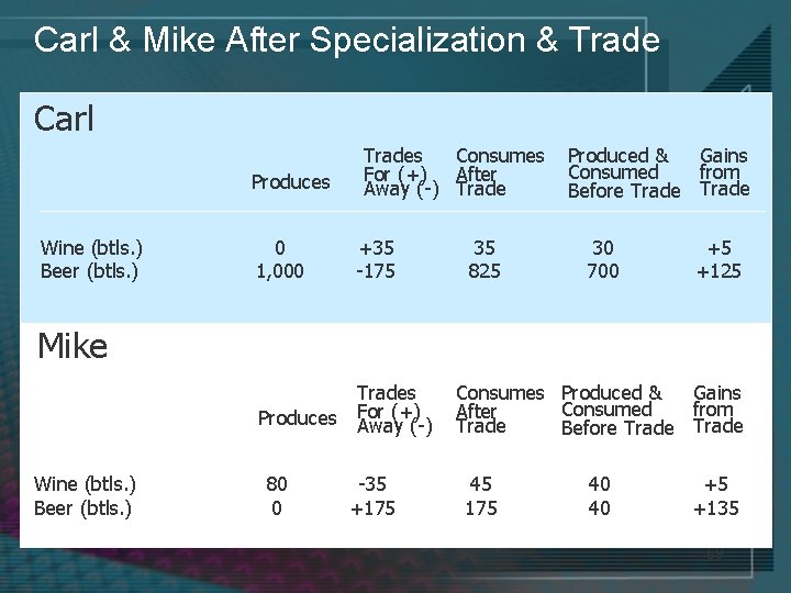
Carl & Mike After Specialization & Trade Carl Produces Wine (btls. ) Beer (btls. ) Trades Consumes For (+) After Away (-) Trade 0 1, 000 +35 -175 Produces Trades For (+) Away (-) 35 825 Produced & Gains Consumed from Before Trade 30 700 +5 +125 Mike Wine (btls. ) Beer (btls. ) 80 0 -35 +175 Consumes Produced & Gains Consumed from After Trade Before Trade 45 175 40 40 +5 +135 69

Mike’s Production Possibilities After Trade Bottles of beer Mike produces 80 wine and then trades 35 wine for 175 beer, leaving him with 45 wine and 175 beer, point D 175 A 80 40 • B • • D Consumption after trade 40 45 C • 80 Bottles of wine 70

Carl’s Production Possibilities/ Opportunity Costs, After Trade Bottles of beer • 100 A Carl produces 1000 beer and trades 175 beer to Mike for 35 wine, leaving him with 825 beer and 35 beer, point D • D 825 700 Consumption after trade B • C 0 30 35 • 100 Bottles of wine 71

Absolute Advantage • When a producer with of set of inputs can produce more output than another with the same inputs, the first producer has an absolute advantage in production of the output. • Carl has an absolute advantage in the production of both wine and beer. 72

Gains from Specialization and Trade • Specialization produces gains for both traders, even when one trader enjoys an absolute advantage in both endeavors. • Unless two people/firms/countries have IDENTICAL opportunity costs, Trade is always beneficial 73

Why No Free Trade? 1) Misunderstanding: people misunderstand the facts or hold to political or ideological dogma, or confuse voluntary jobs with enforced slavery 2) Short-run effects: in the SHORT-RUN, there may be some unpopular adjustments: a) Richer, developed countries may lose jobs to developing countries with a comparative advantage b) Poorer, developing countries may have shortrun environmental damage until the higher incomes lead to environmental protection 74

Chapter 16 Conclusions 1) General equilibrium requires simultaneous equilibrium in multiple markets 2) One change can cause a cascade of changes through markets until a new equilibrium is reached 3) An equilibrium is Pareto Efficient if no other allocation of inputs can make one person better off without making another worse off. 75

Chapter 16 Conclusions 4) Pareto Efficiency requires exchange efficiency (goods can’t be traded), input efficiency (more can’t be produced) and substitution efficiency (substituting production won’t improve outcome) 5) The First Fundamental Theorem of Welfare Economics states that if all perfectly competitive markets exist, allocations are Pareto Efficient 76

Chapter 16 Conclusions 6) The Second Fundamental Theorem of Welfare Economics states that governments can redistribute wealth to reach any pareto efficient outcome 7) Free Trade is always beneficial to all parties 8) Economic truths, when properly applied and explained, can cut through ideologies and make people cry 77