152 Econometric Analysis of Panel Data William Greene

1/52 Econometric Analysis of Panel Data William Greene Department of Economics University of South Florida

2/52 Econometric Analysis of Panel Data 17. Spatial Autoregression and Spatial Autocorelation

3/52 Nonlinear Models with Spatial Data William Greene Stern School of Business, New York University Washington D. C. July 12, 2013

4/52 Applications School District Open Enrollment: A Spatial Multinomial Logit Approach; David Brasington, University of Cincinnati, USA, Alfonso Flores-Lagunes, State University of New York at Binghamton, USA, Ledia Guci, U. S. Bureau of Economic Analysis, USA Smoothed Spatial Maximum Score Estimation of Spatial Autoregressive Binary Choice Panel Models; Jinghua Lei, Tilburg University, The Netherlands Application of Eigenvector-based Spatial Filtering Approach to a Multinomial Logit Model for Land Use Data; Takahiro Yoshida & Morito Tsutsumi, University of Tsukuba, Japan Estimation of Urban Accessibility Indifference Curves by Generalized Ordered Models and Kriging; Abel Brasil, Office of Statistical and Criminal Analysis, Brazil, & Jose Raimundo Carvalho, Universidade Federal do Cear´a, Brazil Choice Set Formation: A Comparative Analysis, Mehran Fasihozaman Langerudi, Mahmoud Javanmardi, Kouros Mohammadian, P. S Sriraj, University of Illinois at Chicago, USA, & Behnam Amini, Imam Khomeini International University, Iran Not including semiparametric and quantile based linear specifications

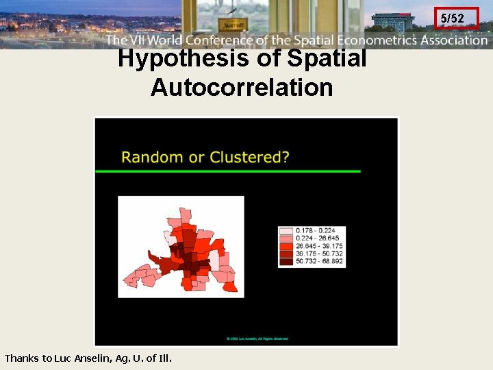
5/52 Hypothesis of Spatial Autocorrelation Thanks to Luc Anselin, Ag. U. of Ill.

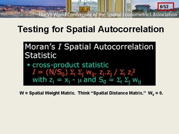
6/52 Testing for Spatial Autocorrelation W = Spatial Weight Matrix. Think “Spatial Distance Matrix. ” W ii = 0.

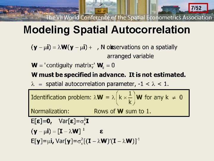
7/52 Modeling Spatial Autocorrelation

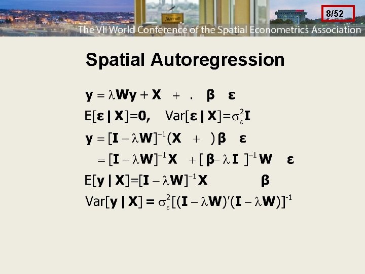
8/52 Spatial Autoregression

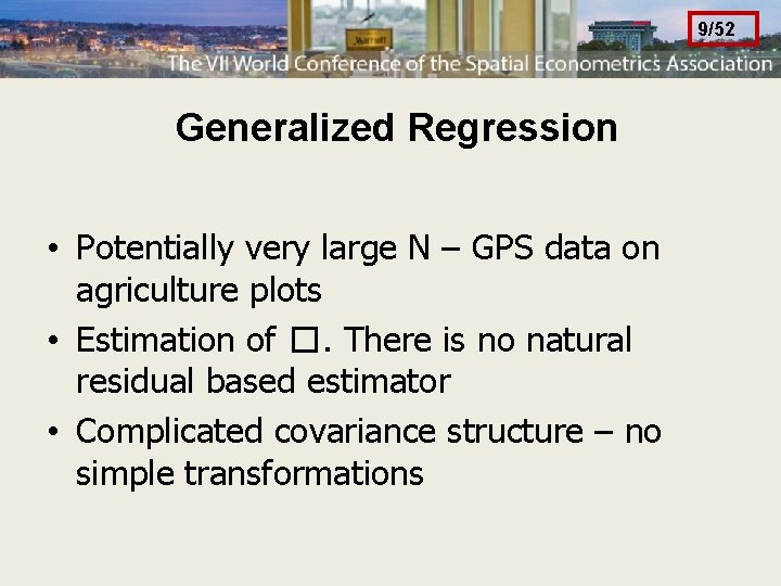
9/52 Generalized Regression • Potentially very large N – GPS data on agriculture plots • Estimation of �. There is no natural residual based estimator • Complicated covariance structure – no simple transformations

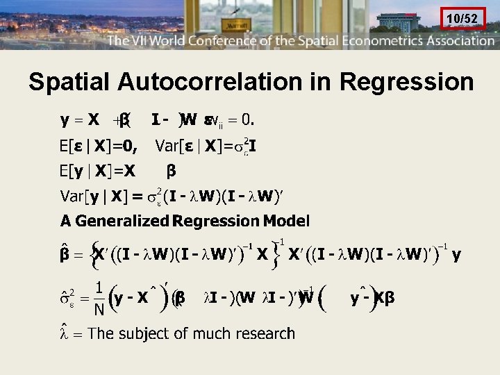
10/52 Spatial Autocorrelation in Regression

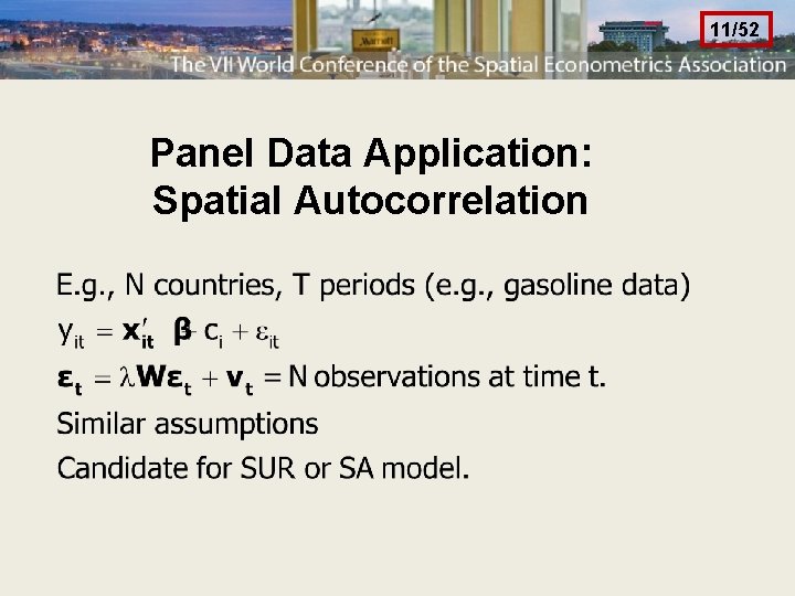
11/52 Panel Data Application: Spatial Autocorrelation

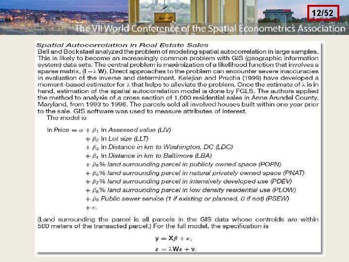
12/52

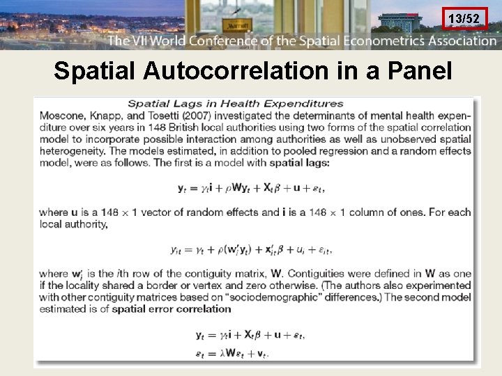
13/52 Spatial Autocorrelation in a Panel

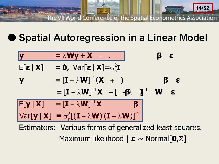
14/52 Spatial Autoregression in a Linear Model

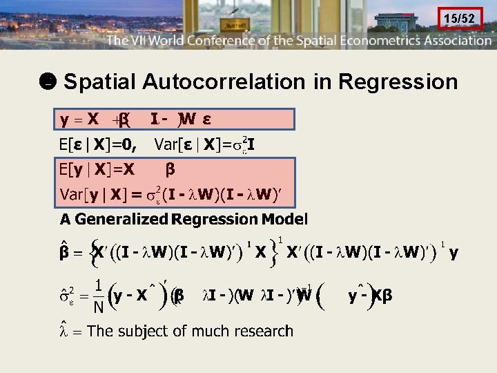
15/52 Spatial Autocorrelation in Regression

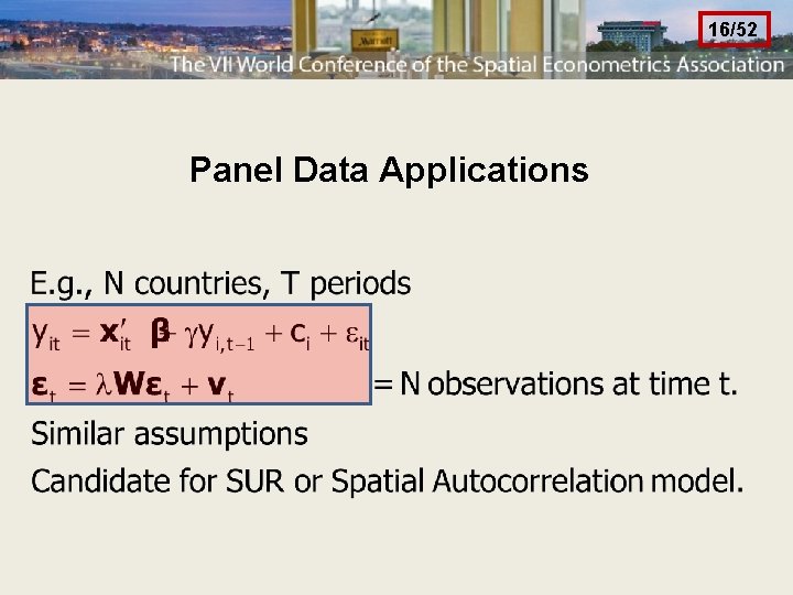
16/52 Panel Data Applications

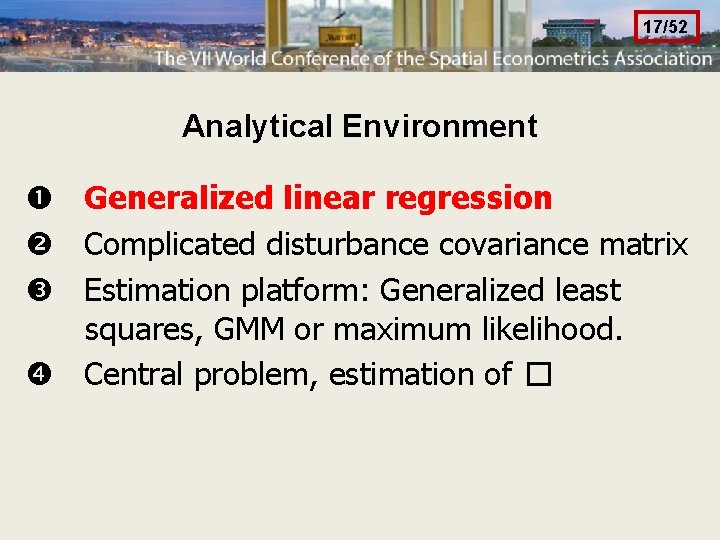
17/52 Analytical Environment Generalized linear regression Complicated disturbance covariance matrix Estimation platform: Generalized least squares, GMM or maximum likelihood. Central problem, estimation of �

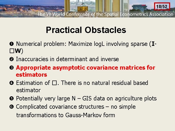
18/52 Practical Obstacles Numerical problem: Maximize log. L involving sparse (I�W) Inaccuracies in determinant and inverse Appropriate asymptotic covariance matrices for estimators Estimation of �. There is no natural residual based estimator Potentially very large N – GIS data on agriculture plots Complicated covariance structures – no simple transformations to Gauss-Markov form

19/52 Binary Outcome: Y=1[New Plant Located in County] Klier and Mc. Millen: Clustering of Auto Supplier Plants in the United States. JBES, 2008

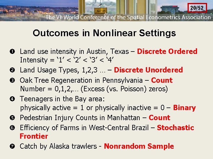
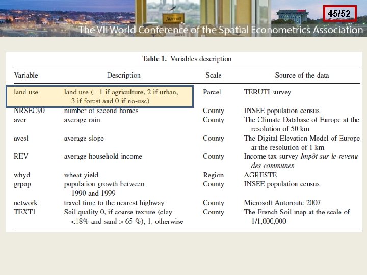
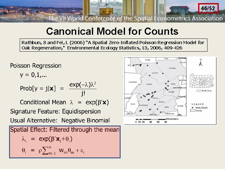
20/52 Outcomes in Nonlinear Settings Land use intensity in Austin, Texas – Discrete Ordered Intensity = ‘ 1’ < ‘ 2’ < ‘ 3’ < ‘ 4’ Land Usage Types, 1, 2, 3 … – Discrete Unordered Oak Tree Regeneration in Pennsylvania – Count Number = 0, 1, 2, … (Excess (vs. Poisson) zeros) Teenagers in the Bay area: physically active = 1 or physically inactive = 0 – Binary Pedestrian Injury Counts in Manhattan – Count Efficiency of Farms in West-Central Brazil – Stochastic Frontier Catch by Alaska trawlers - Nonrandom Sample

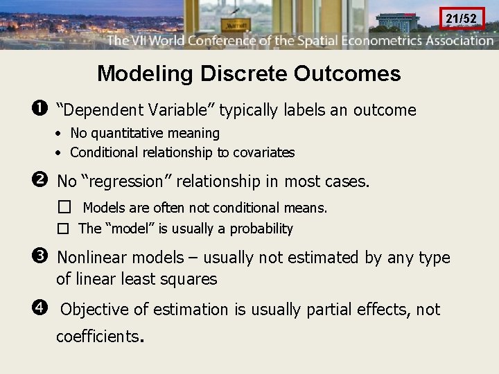
21/52 Modeling Discrete Outcomes “Dependent Variable” typically labels an outcome · No quantitative meaning · Conditional relationship to covariates No “regression” relationship in most cases. � Models are often not conditional means. � The “model” is usually a probability Nonlinear models – usually not estimated by any type of linear least squares Objective of estimation is usually partial effects, not coefficients.

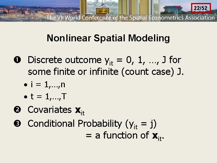
22/52 Nonlinear Spatial Modeling Discrete outcome yit = 0, 1, …, J for some finite or infinite (count case) J. · i = 1, …, n · t = 1, …, T Covariates xit Conditional Probability (yit = j) = a function of xit.

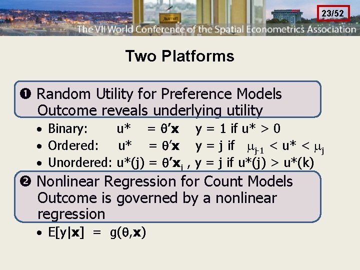
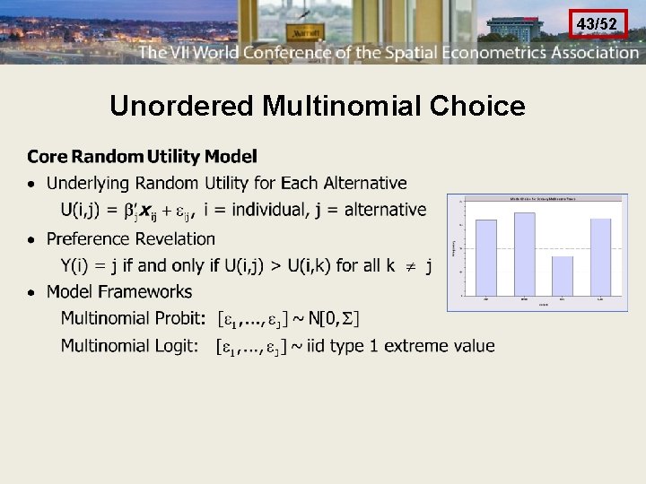
23/52 Two Platforms Random Utility for Preference Models Outcome reveals underlying utility · Binary: u* = ’x y = 1 if u* > 0 · Ordered: u* = ’x y = j if j-1 < u* < j · Unordered: u*(j) = ’xj , y = j if u*(j) > u*(k) Nonlinear Regression for Count Models Outcome is governed by a nonlinear regression · E[y|x] = g( , x)

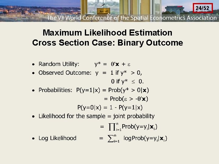
24/52 Maximum Likelihood Estimation Cross Section Case: Binary Outcome

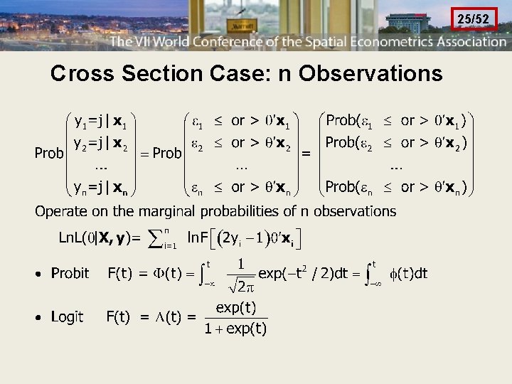
25/52 Cross Section Case: n Observations

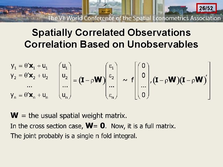
26/52 Spatially Correlated Observations Correlation Based on Unobservables

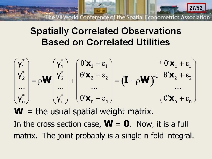
27/52 Spatially Correlated Observations Based on Correlated Utilities

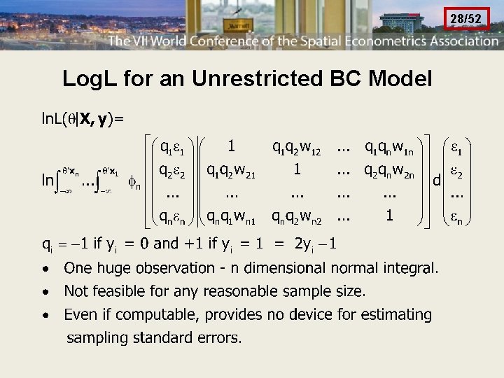
28/52 Log. L for an Unrestricted BC Model

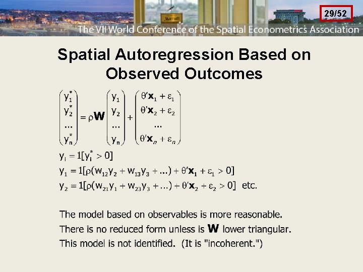
29/52 Spatial Autoregression Based on Observed Outcomes

30/52

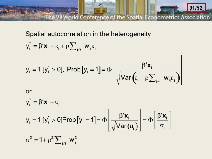
31/52

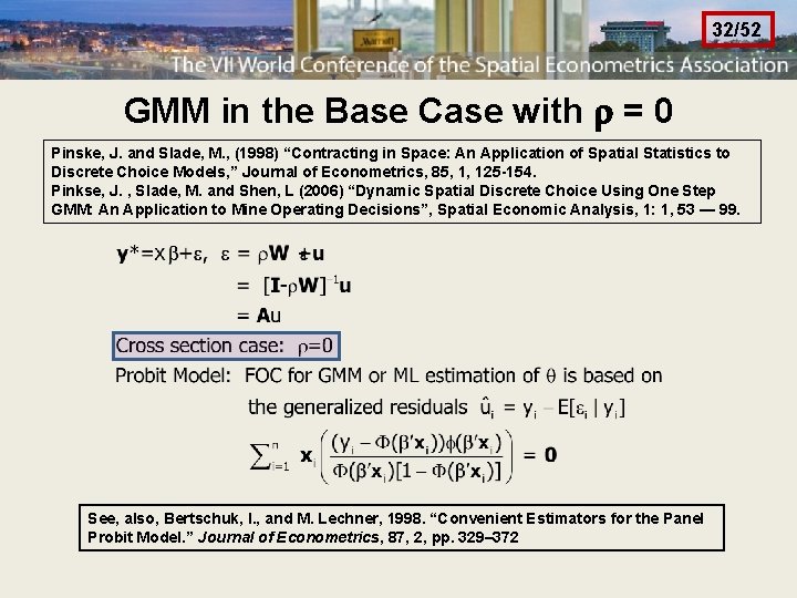
32/52 GMM in the Base Case with = 0 Pinske, J. and Slade, M. , (1998) “Contracting in Space: An Application of Spatial Statistics to Discrete Choice Models, ” Journal of Econometrics, 85, 1, 125 -154. Pinkse, J. , Slade, M. and Shen, L (2006) “Dynamic Spatial Discrete Choice Using One Step GMM: An Application to Mine Operating Decisions”, Spatial Economic Analysis, 1: 1, 53 — 99. See, also, Bertschuk, I. , and M. Lechner, 1998. “Convenient Estimators for the Panel Probit Model. ” Journal of Econometrics, 87, 2, pp. 329– 372

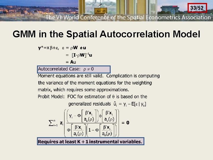
33/52 GMM in the Spatial Autocorrelation Model

34/52

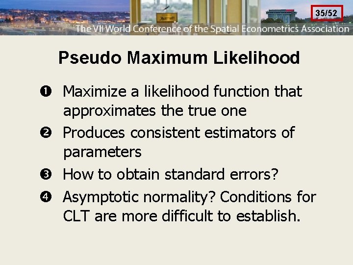
35/52 Pseudo Maximum Likelihood Maximize a likelihood function that approximates the true one Produces consistent estimators of parameters How to obtain standard errors? Asymptotic normality? Conditions for CLT are more difficult to establish.

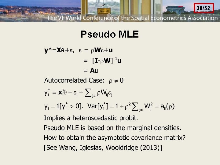
36/52 Pseudo MLE

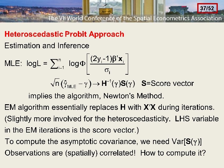
37/52

38/52 See also Arbia, G. , “Pairwise Likelihood Inference for Spatial Regressions Estimated on Very Large Data Sets” Manuscript, Catholic University del Sacro Cuore, Rome, 2012.

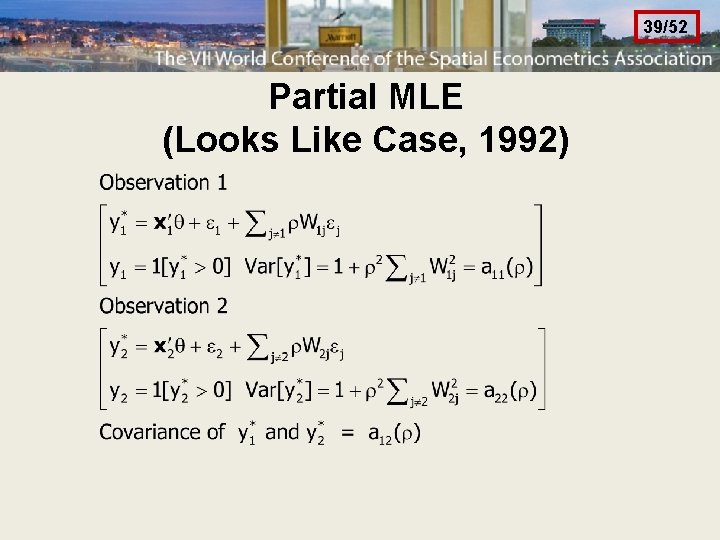
39/52 Partial MLE (Looks Like Case, 1992)

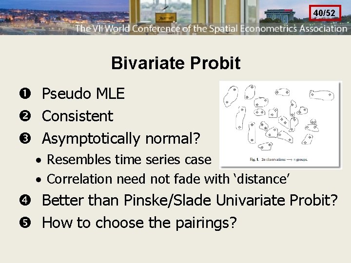
40/52 Bivariate Probit Pseudo MLE Consistent Asymptotically normal? · Resembles time series case · Correlation need not fade with ‘distance’ Better than Pinske/Slade Univariate Probit? How to choose the pairings?

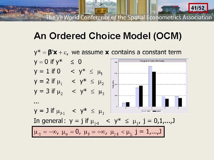
41/52 An Ordered Choice Model (OCM)

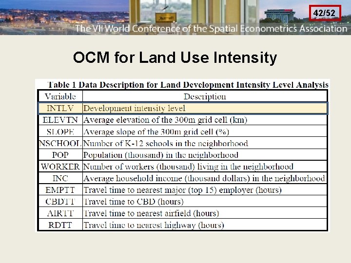
42/52 OCM for Land Use Intensity

43/52 Unordered Multinomial Choice

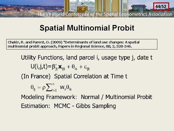
44/52 Spatial Multinomial Probit Chakir, R. and Parent, O. (2009) “Determinants of land use changes: A spatial multinomial probit approach, Papers in Regional Science, 88, 2, 328 -346.

45/52

46/52 Canonical Model for Counts Rathbun, S and Fei, L (2006) “A Spatial Zero-Inflated Poisson Regression Model for Oak Regeneration, ” Environmental Ecology Statistics, 13, 2006, 409 -426

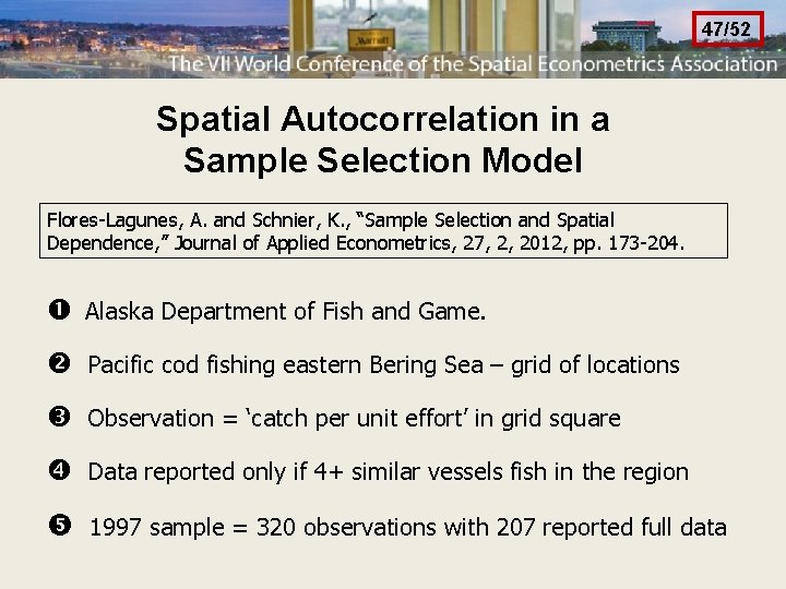
47/52 Spatial Autocorrelation in a Sample Selection Model Flores-Lagunes, A. and Schnier, K. , “Sample Selection and Spatial Dependence, ” Journal of Applied Econometrics, 27, 2, 2012, pp. 173 -204. Alaska Department of Fish and Game. Pacific cod fishing eastern Bering Sea – grid of locations Observation = ‘catch per unit effort’ in grid square Data reported only if 4+ similar vessels fish in the region 1997 sample = 320 observations with 207 reported full data

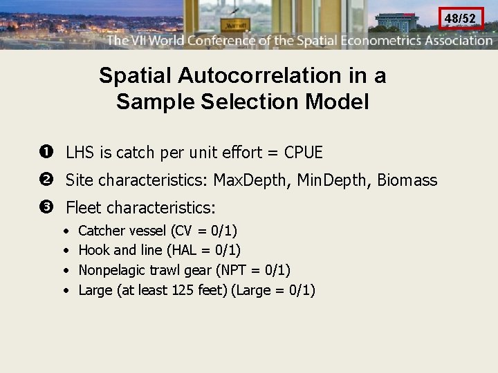
48/52 Spatial Autocorrelation in a Sample Selection Model LHS is catch per unit effort = CPUE Site characteristics: Max. Depth, Min. Depth, Biomass Fleet characteristics: · · Catcher vessel (CV = 0/1) Hook and line (HAL = 0/1) Nonpelagic trawl gear (NPT = 0/1) Large (at least 125 feet) (Large = 0/1)

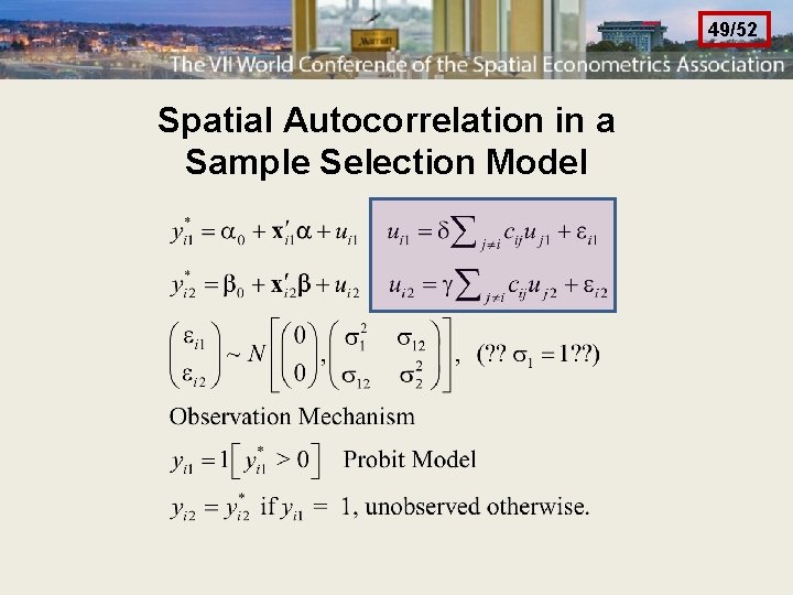
49/52 Spatial Autocorrelation in a Sample Selection Model

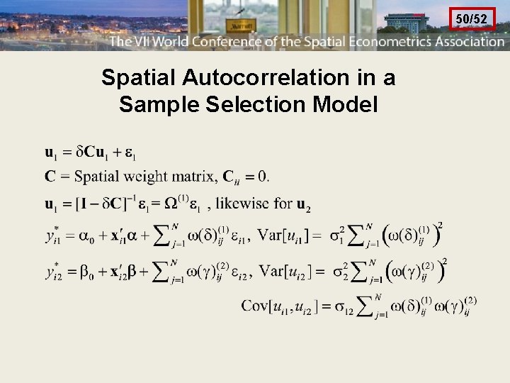
50/52 Spatial Autocorrelation in a Sample Selection Model

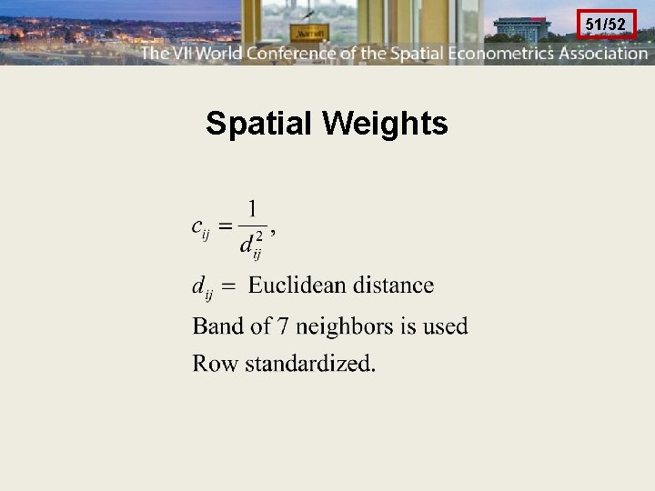
51/52 Spatial Weights

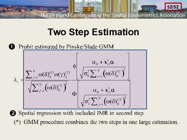
52/52 Two Step Estimation