15 Routing Routing Algorithms n n n Distance

15. Routing & Routing Algorithms n n n Distance vector routing (Bellman-Ford) Link-state routing (Dijkstra) Hierarchical routing Roch Guerin (with adaptations from Jon Turner and John De. Hart, and material from Kurose and Ross)

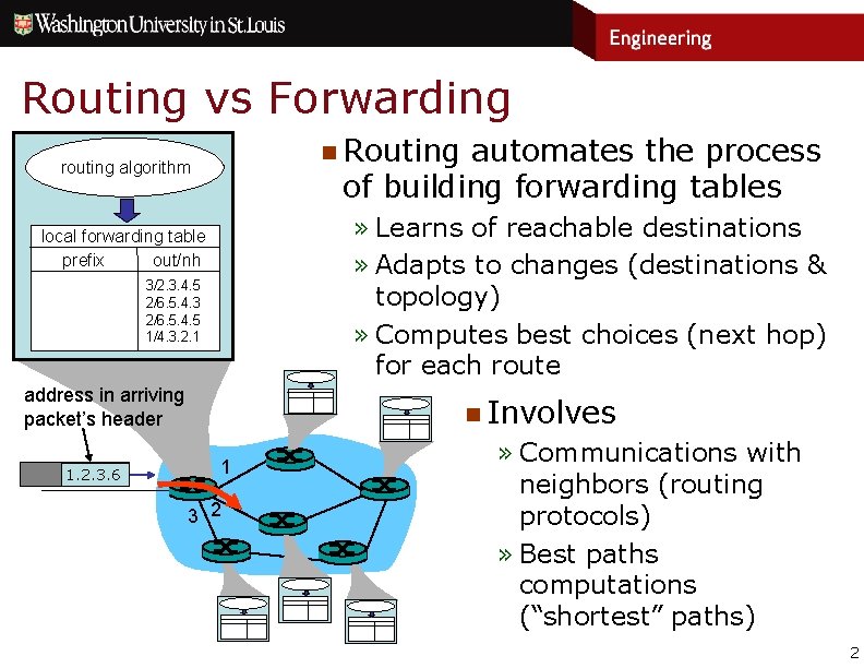
Routing vs Forwarding n Routing automates the process of building forwarding tables routing algorithm » Learns of reachable destinations » Adapts to changes (destinations & topology) » Computes best choices (next hop) for each route local forwarding table prefix out/nh 1. 2. 0. 0/16 3/2. 3. 4. 5 1. 2. 3. 0/24 2/6. 5. 4. 3 3. 2. 1. 0/24 2/6. 5. 4. 5 4. 0. 0. 0/8 1/4. 3. 2. 1 address in arriving packet’s header 1. 2. 3. 6 n Involves 1 3 2 » Communications with neighbors (routing protocols) » Best paths computations (“shortest” paths) 2

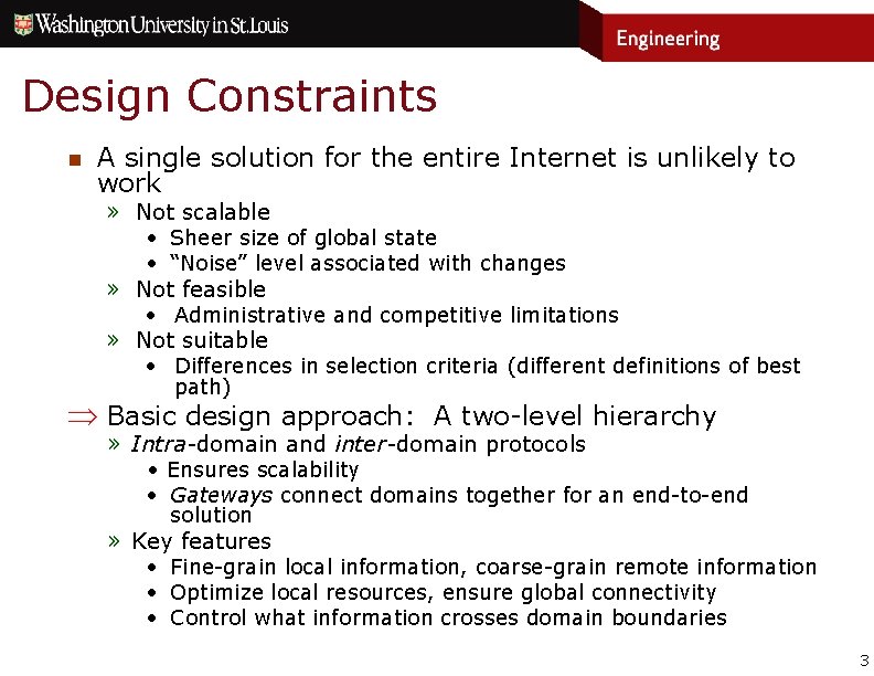
Design Constraints n A single solution for the entire Internet is unlikely to work » Not scalable • Sheer size of global state • “Noise” level associated with changes » Not feasible • Administrative and competitive limitations » Not suitable • Differences in selection criteria (different definitions of best path) Basic design approach: A two-level hierarchy » Intra-domain and inter-domain protocols • Ensures scalability • Gateways connect domains together for an end-to-end solution » Key features • Fine-grain local information, coarse-grain remote information • Optimize local resources, ensure global connectivity • Control what information crosses domain boundaries 3

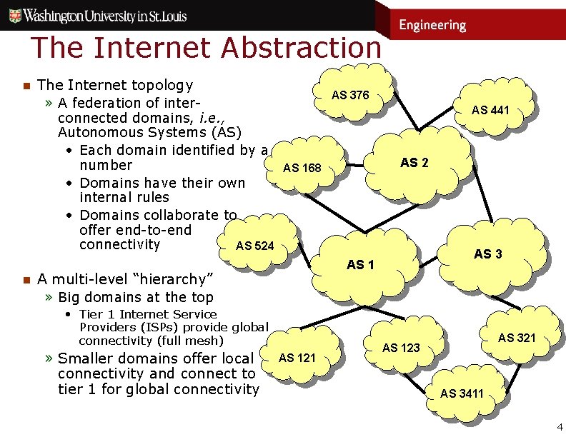
The Internet Abstraction n The Internet topology » A federation of inter- AS 376 AS 441 connected domains, i. e. , Autonomous Systems (AS) • Each domain identified by a number AS 168 • Domains have their own internal rules • Domains collaborate to offer end-to-end connectivity AS 524 n AS 3 AS 1 A multi-level “hierarchy” » Big domains at the top • Tier 1 Internet Service Providers (ISPs) provide global connectivity (full mesh) » Smaller domains offer local connectivity and connect to tier 1 for global connectivity AS 2 AS 121 AS 321 AS 123 AS 3411 4

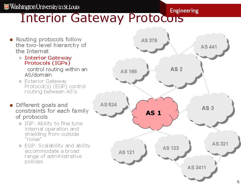
Routing Protocols n A two-level hierarchy for routing protocols AS 376 AS 441 » Interior Gateway Protocols (IGP) control routing within an AS/domain » Exterior Gateway Protocols (EGP) control routing between AS’s n Different goals and constraints for each family of protocols » IGP: Ability to fine tune internal operation and shielding from outside “noise” » EGP: Scalability and ability to accommodate a broad range of administrative policies AS 2 AS 168 AS 524 AS 3 AS 121 AS 321 AS 123 AS 3411 5

Interior Gateway Protocols n Routing protocols follow the two-level hierarchy of the Internet AS 376 AS 441 » Interior Gateway Protocols (IGPs) control routing within an AS/domain » Exterior Gateway Protocol(s) (EGP) control routing between AS’s n Different goals and constraints for each family of protocols » IGP: Ability to fine tune internal operation and shielding from outside “noise” » EGP: Scalability and ability accommodate a broad range of administrative policies AS 2 AS 168 AS 524 AS 3 AS 121 AS 321 AS 123 AS 3411 6

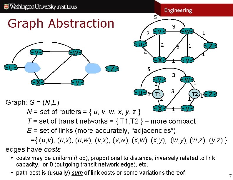
5 Graph Abstraction 2 v u z x y 2 2 w 3 x 5 v 3 1 3 2 u 2 T 1 2 w 1 z 1 1 y w 1 3 1 T 2 1 z Graph: G = (N, E) x 1 y N = set of routers = { u, v, w, x, y, z } T = set of transit networks = { T 1, T 2 } – more compact E = set of links (more accurately, “adjacencies”) ={ (u, v), (u, x), (u, w), (v, x), (v, w), (x, y), (w, z), (y, z) } edges have costs • costs may be uniform (hop), proportional to distance, inversely related to link capacity, or 0 (outgoing transit network edge), etc. • path cost is (usually) sum of link costs or some variations thereof 7

IGP Design Goals n Design parameters 1. Network resources (bandwidth) 2. Router resources – Memory (size of routing table and supporting data structures) – Communication (number and frequency of control messages) – Processing (handling messages & computing forwarding decisions) n Design goals » Correctness • Avoid black holes (unable to reachable destination) • Prevent or recover from loops (inconsistencies across routers) » Stability – Short reaction time to changes, but robustness to frequent changes – Efficiency – Best possible paths (according to some metric) 8

General Design Choices n How are routes learned and forwarding decisions computed? – Centralized vs. distributed - Centralized is simpler but may not scale and more prone to failure - Not just server failure, but more importantly failure to learn about changes - Distributed requires collaboration between routers and has more complex transient behavior (not everyone decides or knows the same thing at the same time) - n More complex ways for things to break, but more options to fix broken things… Assuming a distributed solution: Who computes what and how? - Distance vector protocols – Everyone computes partial results and exchange them to obtain a full answer – Efficiency and scalability benefits, but dependencies on other lengthens reactions - Link state protocols - Everyone individually computes the full answer - Greater overhead, but inherent parallelism of computation yields faster reactions n What is a good path? – What metrics to optimize (hop count, bandwidth, delay, etc. )? – Static vs. dynamic metrics? 9

IGP Summary n Main responsibilities 1) Discover reachable destinations 2) Determine best way to get to reachable destinations – shortest path computation 3) Detect changes to 1) and 2) and update local state • • n Changes to reachability affect best matches for packets Changes to network topology affect where packets are forwarded, and can affect reachability as well IGP protocols differ primarily in the type of shortest path computations they perform » Distance vector (distribute network information and shortest path computations) – Routing Information Protocol V 2 (RIP 2) – Obsolete – Cisco’s Enhanced Interior Gateway Router Protocol (EIGRP) » Link state (distribute network information, perform parallel centralized shortest path computations) – Open Shortest Path First (OSPF) – Intermediate System (IS-IS) 10

Distance Vector Protocols n Iterative procedure to build and update routing tables » Neighbors exchange what they can reach and at what cost • Progressive discovery of reachable destinations • Shortest (lowest cost) path computation based on a distributed (distance vector) computation model n Pros (and cons) of distributed computations » Routers only store routes and associated costs » Routers benefit from each others work (computations) » Routers are only notified of (remote) changes that affect them » But routing convergence can be slow • Serialization of notification and computations • Inconsistencies in knowledge and, therefore, decisions can result in not so transient routing loops or black-holes 11

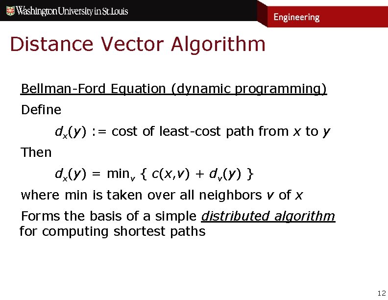
Distance Vector Algorithm Bellman-Ford Equation (dynamic programming) Define dx(y) : = cost of least-cost path from x to y Then dx(y) = minv { c(x, v) + dv(y) } where min is taken over all neighbors v of x Forms the basis of a simple distributed algorithm for computing shortest paths 12

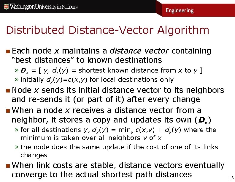
Distributed Distance-Vector Algorithm n Each node x maintains a distance vector containing “best distances” to known destinations » Dx = [ y, dx(y) = shortest known distance from x to y ] » initially dx(y)=c(x, y) for local destinations only n Node x sends its initial distance vector to its neighbors and re-sends it (or part of it) after every change n When a node x receives a distance vector from a neighbor, it stores a copy and updates its own (Dx) » for all destinations y, dx(y) = minv c(x, v) + dv(y) where the minimum is taken over all neighbors v of x » the node does the same update if the cost of one of its links changes n When link costs are stable, distance vectors eventually converge to the actual shortest path distances 13

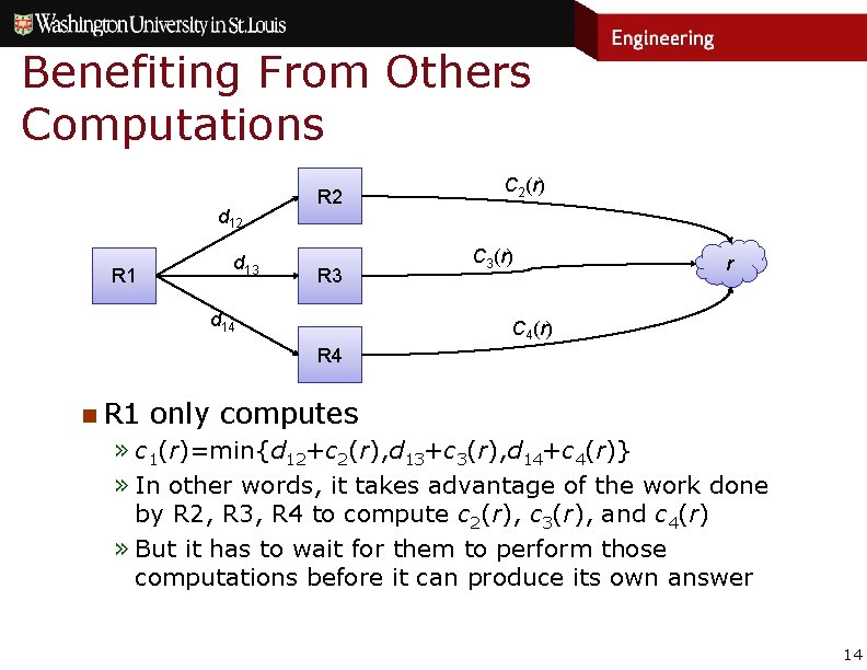
Benefiting From Others Computations d 12 R 1 d 13 R 2 R 3 d 14 C 2(r) C 3(r) r C 4(r) R 4 n R 1 only computes » c 1(r)=min{d 12+c 2(r), d 13+c 3(r), d 14+c 4(r)} » In other words, it takes advantage of the work done by R 2, R 3, R 4 to compute c 2(r), c 3(r), and c 4(r) » But it has to wait for them to perform those computations before it can produce its own answer 14

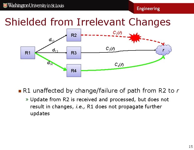
Shielded from Irrelevant Changes d 12 R 1 d 13 R 2 R 3 d 14 C 2(r) C 3(r) r C 4(r) R 4 n R 1 unaffected by change/failure of path from R 2 to r » Update from R 2 is received and processed, but does not result in changes, i. e. , R 1 does not propagate further updates 15

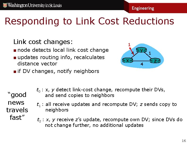
Responding to Link Cost Reductions Link cost changes: ■ node detects local link cost change ■ updates routing info, recalculates distance vector ■ if DV changes, notify neighbors “good news travels fast” 1 4 x y 4 1 z t 0 : x, y detect link-cost change, recompute their DVs, and send copies to neighbors t 1 : all receive updates and recompute DV; z sends copy to neighbors t 2 : x, y receive z’s update, recompute own DV; since DVs do not change further, no additional updates 16

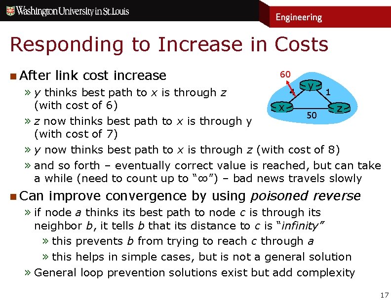
Responding to Increase in Costs n After link cost increase 60 y 4 1 » y thinks best path to x is through z (with cost of 6) x z 50 » z now thinks best path to x is through y (with cost of 7) » y now thinks best path to x is through z (with cost of 8) » and so forth – eventually correct value is reached, but can take a while (need to count up to “∞”) – bad news travels slowly n Can improve convergence by using poisoned reverse » if node a thinks its best path to node c is through its neighbor b, it tells b that its distance to c is “infinity” » this prevents b from trying to reach c through a » this helps in simple cases, but is not a general solution » General loop prevention solutions exist but add complexity 17

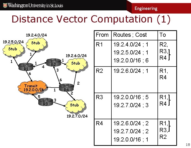
Distance Vector Computation (1) 19. 2. 4. 0/24 19. 2. 5. 0/24 Stub 1 1 1 R 1 4 1 R 2 5 R 3 1 3 R 1 19. 2. 4. 0/24 ; 1 19. 2. 5. 0/24 ; 1 19. 2. 0. 0/16 ; 6 R 2, R 3, R 4 R 2 19. 2. 6. 0/24 ; 1 R 1, R 4 R 3 19. 2. 0. 0/16 ; 5 19. 2. 7. 0/24 ; 3 R 1, R 4 19. 2. 6. 0/24 ; 2 19. 2. 7. 0/24 ; 2 19. 2. 0. 0/16 ; 1 R 1, R 3, R 2 Stub 6 Transit 19. 2. 0. 0/16 To 19. 2. 6. 0/24 3 6 From Routes ; Cost 2 R 4 2 Stub 19. 2. 7. 0/24 18

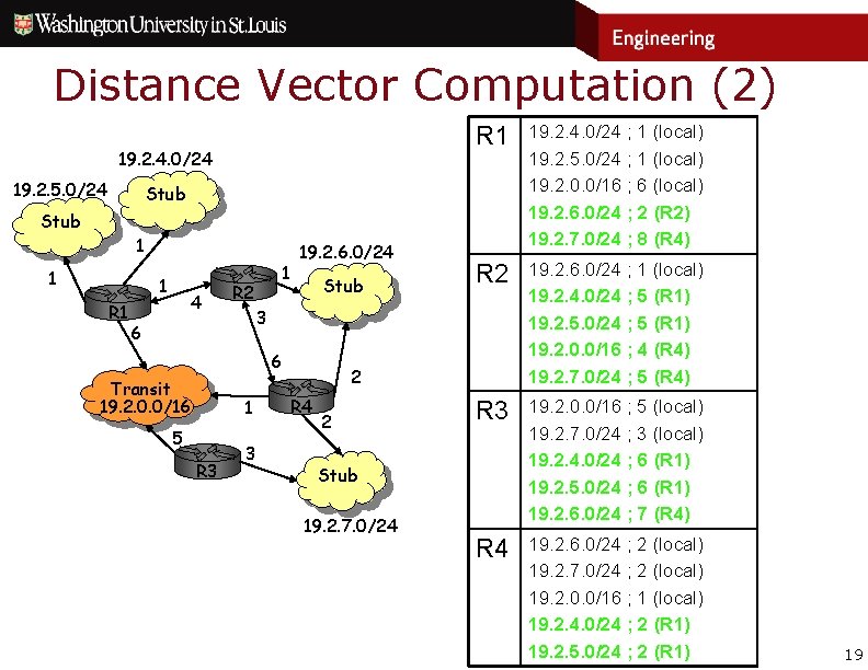
Distance Vector Computation (2) 19. 2. 4. 0/24 19. 2. 5. 0/24 R 1 19. 2. 4. 0/24 ; 1 (local) 19. 2. 5. 0/24 ; 1 (local) 19. 2. 0. 0/16 ; 6 (local) 19. 2. 6. 0/24 ; 2 (R 2) 19. 2. 7. 0/24 ; 8 (R 4) R 2 19. 2. 6. 0/24 ; 1 (local) 19. 2. 4. 0/24 ; 5 (R 1) 19. 2. 5. 0/24 ; 5 (R 1) 19. 2. 0. 0/16 ; 4 (R 4) 19. 2. 7. 0/24 ; 5 (R 4) R 3 19. 2. 0. 0/16 ; 5 (local) 19. 2. 7. 0/24 ; 3 (local) 19. 2. 4. 0/24 ; 6 (R 1) 19. 2. 5. 0/24 ; 6 (R 1) 19. 2. 6. 0/24 ; 7 (R 4) R 4 19. 2. 6. 0/24 ; 2 (local) 19. 2. 7. 0/24 ; 2 (local) 19. 2. 0. 0/16 ; 1 (local) 19. 2. 4. 0/24 ; 2 (R 1) 19. 2. 5. 0/24 ; 2 (R 1) Stub 1 1 1 R 1 4 1 R 2 19. 2. 6. 0/24 Stub 3 6 6 Transit 19. 2. 0. 0/16 1 5 R 3 3 2 R 4 2 Stub 19. 2. 7. 0/24 19

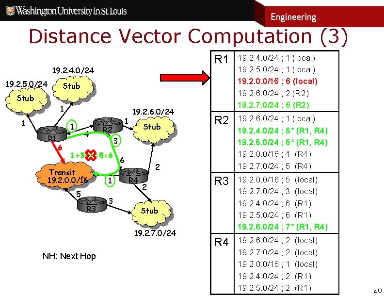
Distance Vector Computation (3) 19. 2. 4. 0/24 19. 2. 5. 0/24 R 1 19. 2. 4. 0/24 ; 1 (local) 19. 2. 5. 0/24 ; 1 (local) 19. 2. 0. 0/16 ; 6 (local) 19. 2. 6. 0/24 ; 2 (R 2) 19. 2. 7. 0/24 ; 6 (R 2) R 2 19. 2. 6. 0/24 ; 1 (local) 19. 2. 4. 0/24 ; 5* (R 1, R 4) 19. 2. 5. 0/24 ; 5* (R 1, R 4) 19. 2. 0. 0/16 ; 4 (R 4) 19. 2. 7. 0/24 ; 5 (R 4) R 3 19. 2. 0. 0/16 ; 5 (local) 19. 2. 7. 0/24 ; 3 (local) 19. 2. 4. 0/24 ; 6 (R 1) 19. 2. 5. 0/24 ; 6 (R 1) 19. 2. 6. 0/24 ; 7* (R 1, R 4) R 4 19. 2. 6. 0/24 ; 2 19. 2. 7. 0/24 ; 2 19. 2. 0. 0/16 ; 1 19. 2. 4. 0/24 ; 2 19. 2. 5. 0/24 ; 2 Stub 1 1 1 R 1 6 4 R 2 5 R 3 Stub 3 1+3+1=5<6 Transit 19. 2. 0. 0/16 1 19. 2. 6. 0/24 1 3 6 2 R 4 2 Stub 19. 2. 7. 0/24 NH: Next Hop (local) (R 1) 20

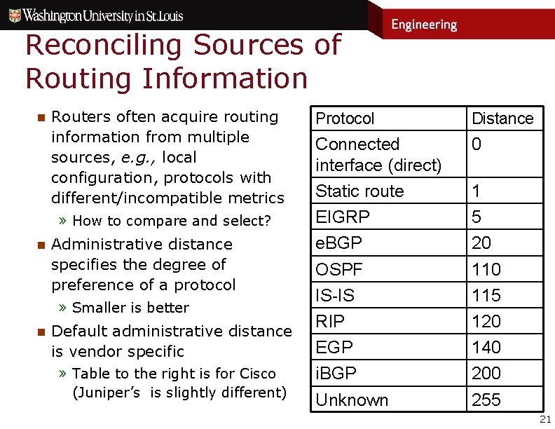
Reconciling Sources of Routing Information n Routers often acquire routing information from multiple sources, e. g. , local configuration, protocols with different/incompatible metrics » How to compare and select? n Administrative distance specifies the degree of preference of a protocol » Smaller is better n Default administrative distance is vendor specific » Table to the right is for Cisco (Juniper’s is slightly different) Protocol Distance Connected interface (direct) Static route EIGRP e. BGP OSPF IS-IS RIP EGP i. BGP Unknown 0 1 5 20 115 120 140 200 255 21

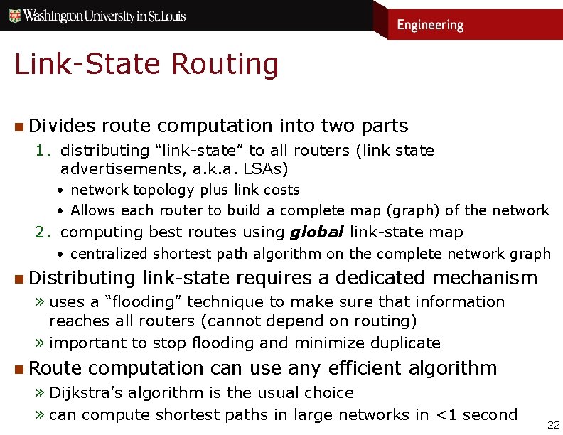
Link-State Routing n Divides route computation into two parts 1. distributing “link-state” to all routers (link state advertisements, a. k. a. LSAs) • network topology plus link costs • Allows each router to build a complete map (graph) of the network 2. computing best routes using global link-state map • centralized shortest path algorithm on the complete network graph n Distributing link-state requires a dedicated mechanism » uses a “flooding” technique to make sure that information reaches all routers (cannot depend on routing) » important to stop flooding and minimize duplicate n Route computation can use any efficient algorithm » Dijkstra’s algorithm is the usual choice » can compute shortest paths in large networks in <1 second 22

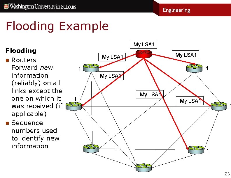
Flooding Example Flooding n Routers Forward new information (reliably) on all links except the on which it was received (if applicable) n Sequence numbers used to identify new information My LSA 1 My LSA 1 1 1 23

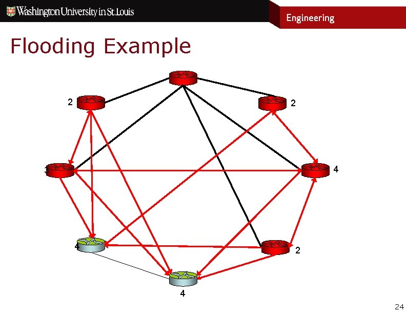
Flooding Example 2 2 4 3 4 24

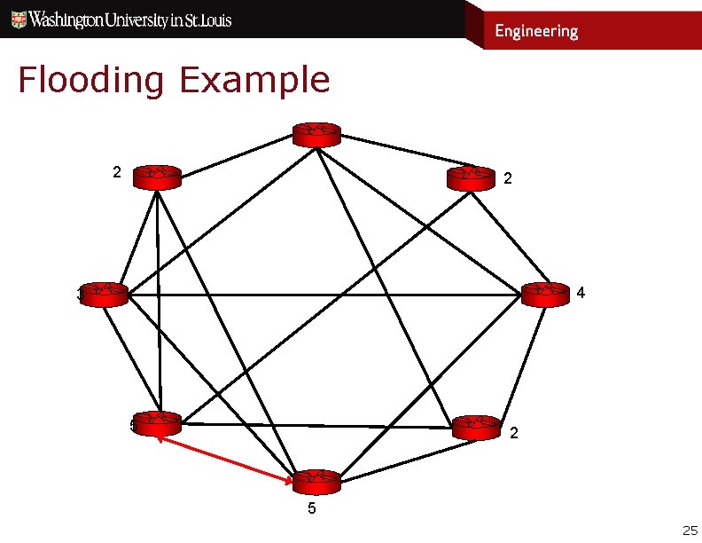
Flooding Example 2 2 4 3 5 25

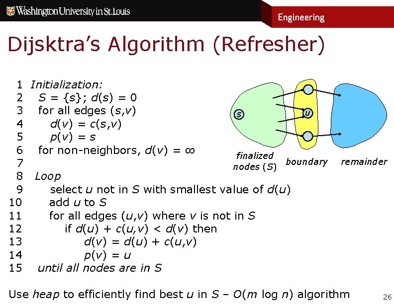
Dijsktra’s Algorithm (Refresher) 1 Initialization: 2 S = {s}; d(s) = 0 3 for all edges (s, v) u s 4 d(v) = c(s, v) 5 p(v) = s 6 for non-neighbors, d(v) = ∞ finalized boundary 7 nodes (S) 8 Loop 9 select u not in S with smallest value of d(u) 10 add u to S 11 for all edges (u, v) where v is not in S 12 if d(u) + c(u, v) < d(v) then 13 d(v) = d(u) + c(u, v) 14 p(v) = u 15 until all nodes are in S remainder Use heap to efficiently find best u in S – O(m log n) algorithm 26

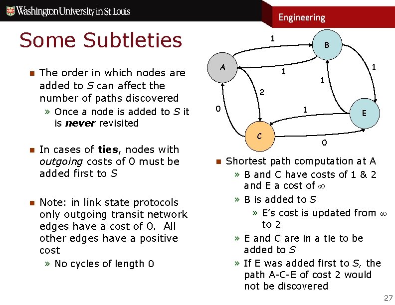
Some Subtleties n The order in which nodes are added to S can affect the number of paths discovered » Once a node is added to S it 1 A B 1 1 1 2 0 1 E is never revisited C n n In cases of ties, nodes with outgoing costs of 0 must be added first to S Note: in link state protocols only outgoing transit network edges have a cost of 0. All other edges have a positive cost » No cycles of length 0 n 0 Shortest path computation at A » B and C have costs of 1 & 2 and E a cost of ∞ » B is added to S » E’s cost is updated from ∞ to 2 » E and C are in a tie to be added to S » If E was added first to S, the path A-C-E of cost 2 would not be discovered 27

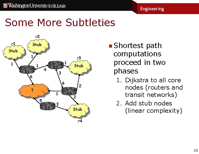
Some More Subtleties r 2 r 1 n Shortest Stub 1 1 1 R 1 4 r 3 1 R 2 Stub 3 6 6 T 1 5 R 3 3 2 R 4 2 Stub path computations proceed in two phases 1. Dijkstra to all core nodes (routers and transit networks) 2. Add stub nodes (linear complexity) r 4 28

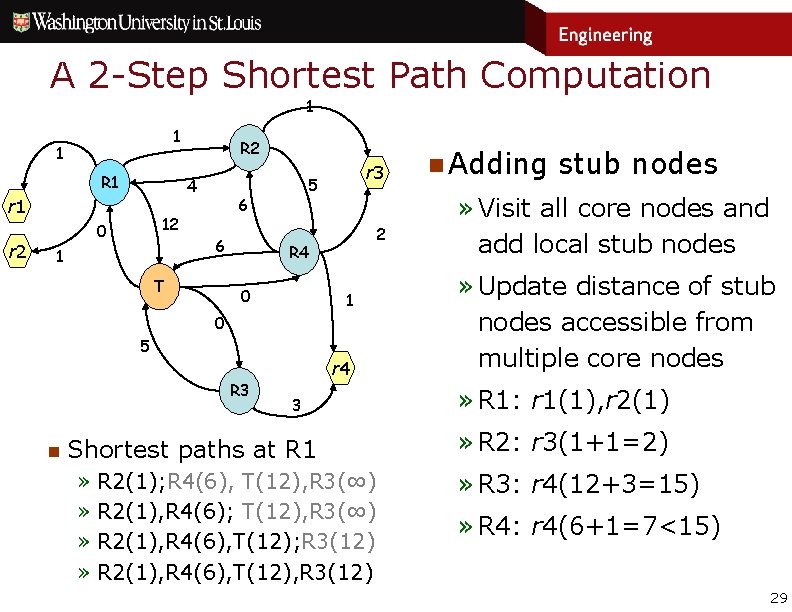
A 2 -Step Shortest Path Computation 1 1 1 R 1 4 r 1 r 2 R 2 0 6 1 5 6 12 T r 3 2 R 4 0 1 0 5 r 4 R 3 n 3 Shortest paths at R 1 » R 2(1); R 4(6), T(12), R 3(∞) » R 2(1), R 4(6); T(12), R 3(∞) » R 2(1), R 4(6), T(12); R 3(12) » R 2(1), R 4(6), T(12), R 3(12) n Adding stub nodes » Visit all core nodes and add local stub nodes » Update distance of stub nodes accessible from multiple core nodes » R 1: r 1(1), r 2(1) » R 2: r 3(1+1=2) » R 3: r 4(12+3=15) » R 4: r 4(6+1=7<15) 29

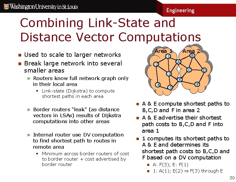
Combining Link-State and Distance Vector Computations n n Area 1 Used to scale to larger networks Break large network into several smaller areas • Minimum across border routers of cost to border router + cost advertised by border router A 2 C 3 D E 4 • Link-state (Dijkstra) to compute shortest paths in each area » Internal router use DV computation to find shortest path to routes in remote area B 1 » Routers know full network graph only in their local area » Border routers “leak” (as distance vectors in LSAs) results of Dijkstra computations into other areas Area 2 n n n 5 F A & E compute shortest paths to B, C, D and F in area 2 A & E advertise their shortest path costs to B, C, D and F into area 1 1 computes its shortest paths to A & E and determines its shortest path costs to B, C, D and F based on a DV computation n n A: F(3); E: F(1) 1: A(1); E(2) F(3) through E 30

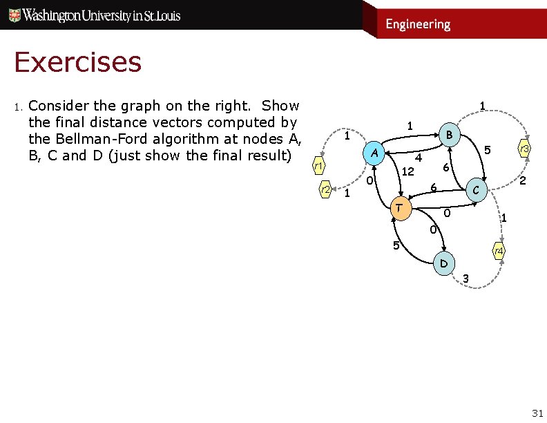
Exercises 1. Consider the graph on the right. Show the final distance vectors computed by the Bellman-Ford algorithm at nodes A, B, C and D (just show the final result) 1 1 1 A r 1 r 2 1 12 0 B 5 4 r 3 6 6 T 2 C 0 1 0 5 r 4 D 3 31

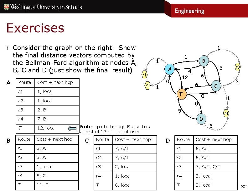
Exercises 1. A B Consider the graph on the right. Show the final distance vectors computed by the Bellman-Ford algorithm at nodes A, B, C and D (just show the final result) Route Cost + next hop r 1 1, local r 2 1, local r 3 2, B r 4 7, B T 12, local Route Cost + next hop r 1 1 A r 1 r 2 1 12 0 B 5 4 r 3 6 6 T 2 C 0 1 0 5 r 4 D 3 Note: path through B also has a cost of 12 but is not used Route Cost + next hop 7, A/T r 1 6, A/T r 2 7, A/T r 2 6, A/T 1, local r 3 2, local r 3 7, A/T, C/T r 4 6, C r 4 1, local r 4 3, local T 11, C T 6, local T 5, local Route Cost + next hop 5, A r 1 r 2 5, A r 3 C D 32

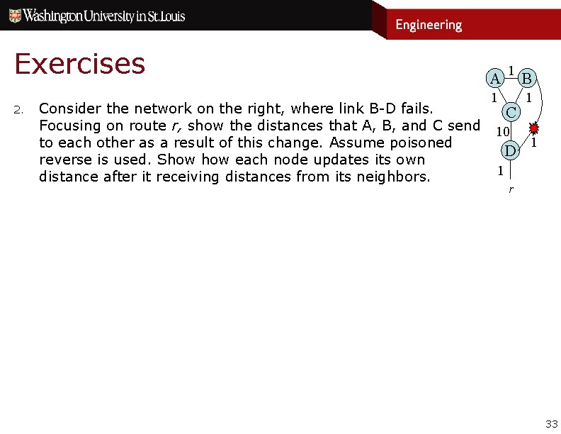
Exercises 2. Consider the network on the right, where link B-D fails. Focusing on route r, show the distances that A, B, and C send to each other as a result of this change. Assume poisoned reverse is used. Show each node updates its own distance after it receiving distances from its neighbors. A 1 1 C 10 D B 1 1 1 r 33

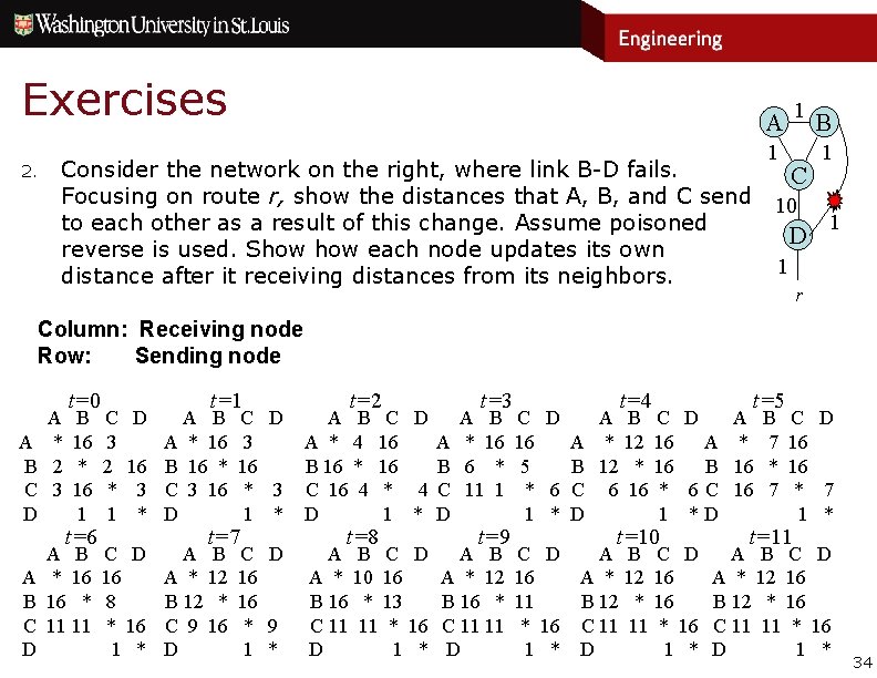
Exercises 2. 1 A Consider the network on the right, where link B-D fails. Focusing on route r, show the distances that A, B, and C send to each other as a result of this change. Assume poisoned reverse is used. Show each node updates its own distance after it receiving distances from its neighbors. 1 C 10 D B 1 1 1 r Column: Receiving node Row: Sending node A A * B 2 C 3 D t=0 B 16 * 16 1 t=6 A B A * 16 B 16 * C 11 11 D C 3 2 * 1 D t=1 A B A * 16 16 B 16 * 3 C 3 16 * D C D 16 8 * 16 1 * t=3 t=8 t=9 C D 3 16 * 3 1 * A B A * 4 B 16 * C 16 4 D C D 16 16 * 9 1 * A B C D A * 10 16 B 16 * 13 C 11 11 * 16 D 1 * t=7 A B A * 12 B 12 * C 9 16 D t=2 C D A B 16 A * 16 16 B 6 * * 4 C 11 1 1 * D A B A * 12 B 16 * C 11 11 D t=4 t=5 t=10 t=11 C D A B 16 A * 12 16 A * 7 5 B 12 * 16 B 16 * * 6 C 6 16 * 6 C 16 7 1 * D 1 *D C D A B C D 16 A * 12 16 11 B 12 * 16 C 11 11 * 16 1 * D 1 * C D 16 16 * 7 1 * A B C D A * 12 16 B 12 * 16 C 11 11 * 16 D 1 * 34

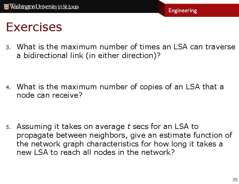
Exercises 3. What is the maximum number of times an LSA can traverse a bidirectional link (in either direction)? 4. What is the maximum number of copies of an LSA that a node can receive? 5. Assuming it takes on average t secs for an LSA to propagate between neighbors, give an estimate function of the network graph characteristics for how long it takes a new LSA to reach all nodes in the network? 35

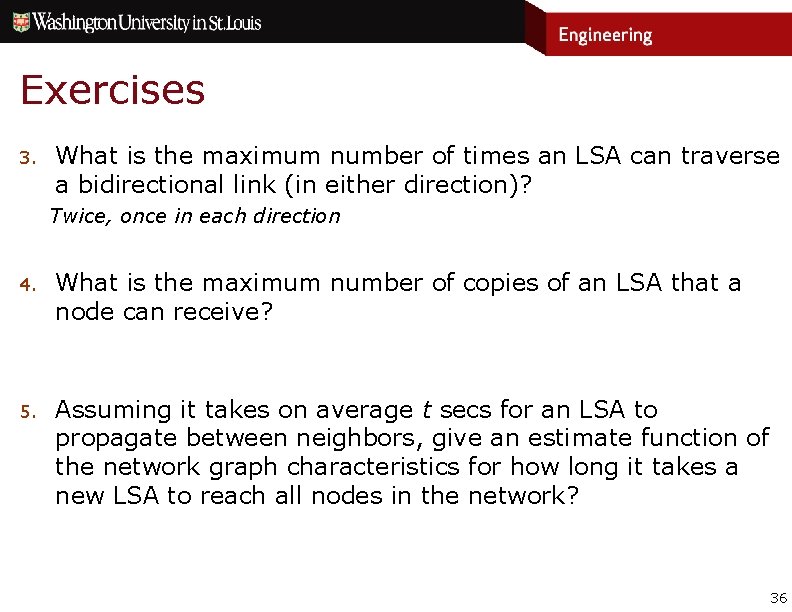
Exercises 3. What is the maximum number of times an LSA can traverse a bidirectional link (in either direction)? Twice, once in each direction 4. What is the maximum number of copies of an LSA that a node can receive? 5. Assuming it takes on average t secs for an LSA to propagate between neighbors, give an estimate function of the network graph characteristics for how long it takes a new LSA to reach all nodes in the network? 36

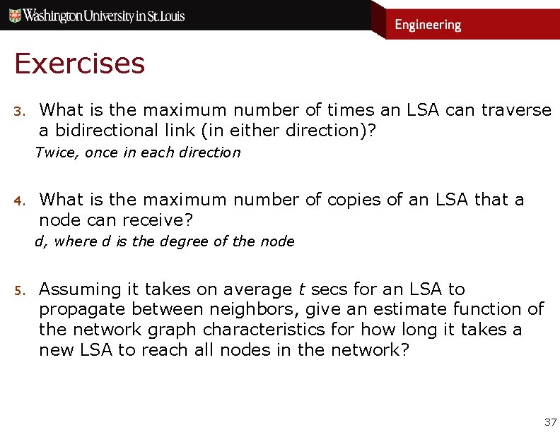
Exercises 3. What is the maximum number of times an LSA can traverse a bidirectional link (in either direction)? Twice, once in each direction 4. What is the maximum number of copies of an LSA that a node can receive? d, where d is the degree of the node 5. Assuming it takes on average t secs for an LSA to propagate between neighbors, give an estimate function of the network graph characteristics for how long it takes a new LSA to reach all nodes in the network? 37

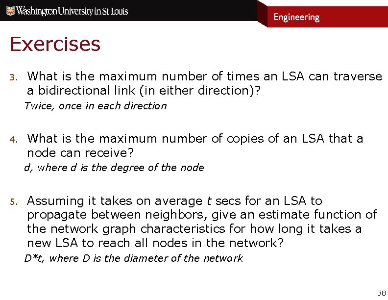
Exercises 3. What is the maximum number of times an LSA can traverse a bidirectional link (in either direction)? Twice, once in each direction 4. What is the maximum number of copies of an LSA that a node can receive? d, where d is the degree of the node 5. Assuming it takes on average t secs for an LSA to propagate between neighbors, give an estimate function of the network graph characteristics for how long it takes a new LSA to reach all nodes in the network? D*t, where D is the diameter of the network 38

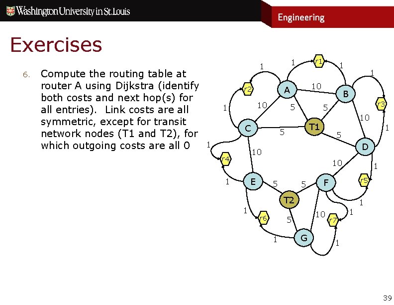
Exercises 6. Compute the routing table at router A using Dijkstra (identify both costs and next hop(s) for all entries). Link costs are all symmetric, except for transit network nodes (T 1 and T 2), for which outgoing costs are all 0 10 1 5 C 1 10 A r 2 1 r 1 1 B r 3 5 10 T 1 5 D 10 r 4 10 E 1 5 5 1 r 5 F T 2 1 r 6 10 5 1 G r 7 1 1 1 39

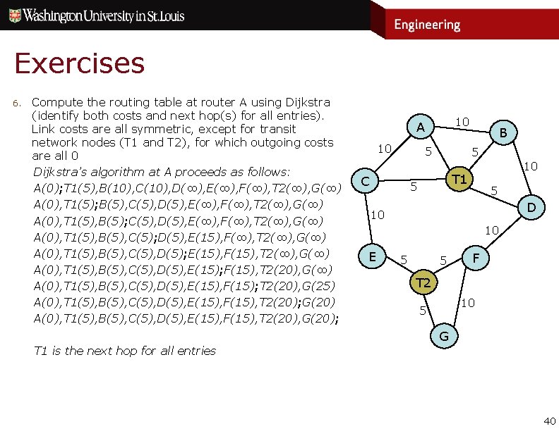
Exercises 6. Compute the routing table at router A using Dijkstra (identify both costs and next hop(s) for all entries). Link costs are all symmetric, except for transit network nodes (T 1 and T 2), for which outgoing costs are all 0 Dijkstra’s algorithm at A proceeds as follows: A(0); T 1(5), B(10), C(10), D(∞), E(∞), F(∞), T 2(∞), G(∞) A(0), T 1(5); B(5), C(5), D(5), E(∞), F(∞), T 2(∞), G(∞) A(0), T 1(5), B(5); C(5), D(5), E(∞), F(∞), T 2(∞), G(∞) A(0), T 1(5), B(5), C(5); D(5), E(15), F(∞), T 2(∞), G(∞) A(0), T 1(5), B(5), C(5), D(5); E(15), F(15), T 2(∞), G(∞) A(0), T 1(5), B(5), C(5), D(5), E(15); F(15), T 2(20), G(∞) A(0), T 1(5), B(5), C(5), D(5), E(15), F(15); T 2(20), G(25) A(0), T 1(5), B(5), C(5), D(5), E(15), F(15), T 2(20); G(20) A(0), T 1(5), B(5), C(5), D(5), E(15), F(15), T 2(20), G(20); T 1 is the next hop for all entries 10 A 10 5 C B 5 10 T 1 5 5 D 10 10 E 5 5 F T 2 10 5 G 40

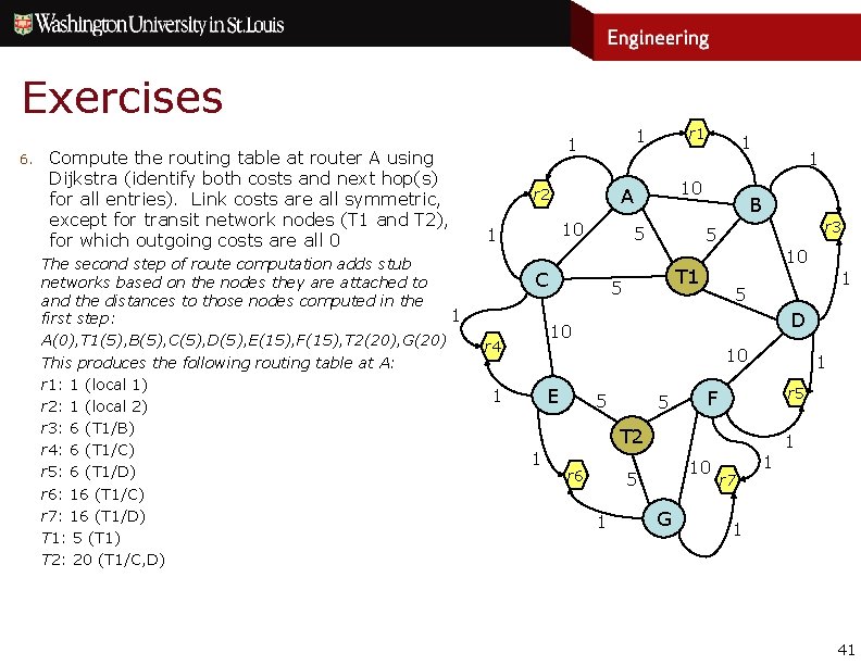
Exercises 6. Compute the routing table at router A using Dijkstra (identify both costs and next hop(s) for all entries). Link costs are all symmetric, except for transit network nodes (T 1 and T 2), for which outgoing costs are all 0 The second step of route computation adds stub networks based on the nodes they are attached to and the distances to those nodes computed in the 1 first step: A(0), T 1(5), B(5), C(5), D(5), E(15), F(15), T 2(20), G(20) This produces the following routing table at A: r 1: 1 (local 1) r 2: 1 (local 2) r 3: 6 (T 1/B) r 4: 6 (T 1/C) r 5: 6 (T 1/D) r 6: 16 (T 1/C) r 7: 16 (T 1/D) T 1: 5 (T 1) T 2: 20 (T 1/C, D) r 1 10 A r 2 10 1 5 C 1 1 B r 3 5 10 T 1 5 D 10 r 4 10 E 1 5 5 1 r 5 F T 2 1 r 6 10 5 1 G r 7 1 1 1 41

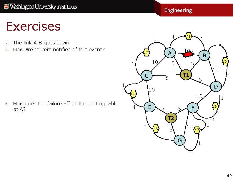
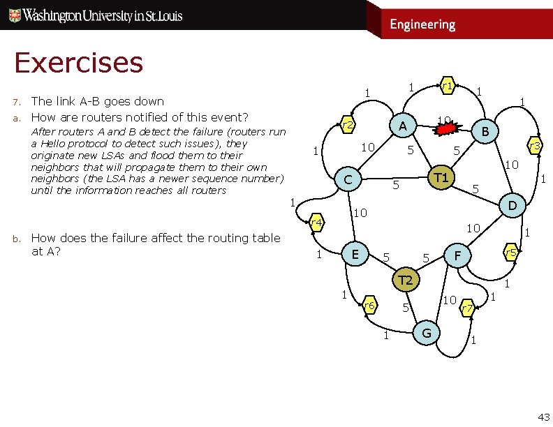
Exercises 7. a. The link A-B goes down How are routers notified of this event? 10 1 5 C How does the failure affect the routing table at A? 1 B r 3 5 10 T 1 5 D 10 r 4 b. 1 10 A r 2 1 r 1 10 E 1 5 5 1 r 5 F T 2 1 r 6 10 5 1 G r 7 1 1 1 42

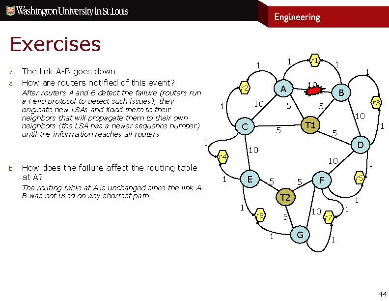
Exercises 7. a. The link A-B goes down How are routers notified of this event? After routers A and B detect the failure (routers run a Hello protocol to detect such issues), they originate new LSAs and flood them to their neighbors that will propagate them to their own neighbors (the LSA has a newer sequence number) until the information reaches all routers 10 1 How does the failure affect the routing table at A? 1 B r 3 5 10 T 1 5 D 10 r 4 b. 5 C 1 10 A r 2 1 r 1 10 E 1 5 5 1 r 5 F T 2 1 r 6 10 5 1 G r 7 1 1 1 43

Exercises 7. a. The link A-B goes down How are routers notified of this event? After routers A and B detect the failure (routers run a Hello protocol to detect such issues), they originate new LSAs and flood them to their neighbors that will propagate them to their own neighbors (the LSA has a newer sequence number) until the information reaches all routers 10 1 How does the failure affect the routing table at A? The routing table at A is unchanged since the link AB was not used on any shortest path. 1 B r 3 5 10 T 1 5 D 10 r 4 b. 5 C 1 10 A r 2 1 r 1 10 E 1 5 5 1 r 5 F T 2 1 r 6 10 5 1 G r 7 1 1 1 44

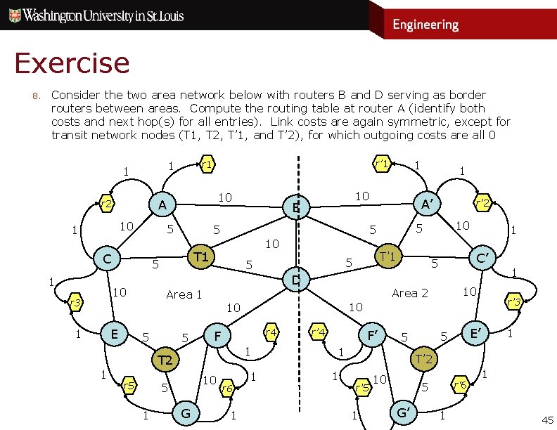
Exercise 8. Consider the two area network below with routers B and D serving as border routers between areas. Compute the routing table at router A (identify both costs and next hop(s) for all entries). Link costs are again symmetric, except for transit network nodes (T 1, T 2, T’ 1, and T’ 2), for which outgoing costs are all 0 10 1 5 C E 1 T 1 D 5 5 r 5 5 1 G r 4 1 1 1 C’ 5 1 10 r’ 3 10 F r 6 10 Area 2 10 10 r'2 5 T’ 1 5 5 1 A’ 5 T 2 1 B 10 Area 1 1 10 5 5 10 r 3 10 A r 2 1 r'1 r 1 1 r’ 4 F’ 1 1 E’ 5 5 1 T’ 2 r’ 5 1 10 r'6 5 G’ 1 1 45

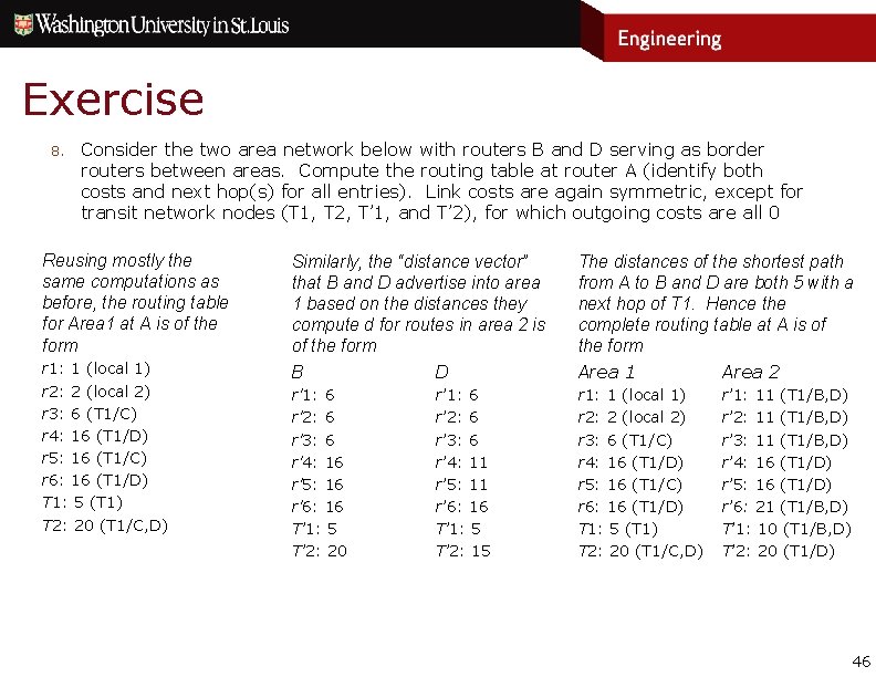
Exercise 8. Consider the two area network below with routers B and D serving as border routers between areas. Compute the routing table at router A (identify both costs and next hop(s) for all entries). Link costs are again symmetric, except for transit network nodes (T 1, T 2, T’ 1, and T’ 2), for which outgoing costs are all 0 Reusing mostly the same computations as before, the routing table for Area 1 at A is of the form r 1: 1 (local 1) r 2: 2 (local 2) r 3: 6 (T 1/C) r 4: 16 (T 1/D) r 5: 16 (T 1/C) r 6: 16 (T 1/D) T 1: 5 (T 1) T 2: 20 (T 1/C, D) Similarly, the “distance vector” that B and D advertise into area 1 based on the distances they compute d for routes in area 2 is of the form B D The distances of the shortest path from A to B and D are both 5 with a next hop of T 1. Hence the complete routing table at A is of the form Area 1 Area 2 r'1: 6 r'2: 6 r'3: 6 r'4: 16 r'5: 16 r'6: 16 T’ 1: 5 T’ 2: 20 r 1: 1 (local 1) r 2: 2 (local 2) r 3: 6 (T 1/C) r 4: 16 (T 1/D) r 5: 16 (T 1/C) r 6: 16 (T 1/D) T 1: 5 (T 1) T 2: 20 (T 1/C, D) r’ 1: 6 r’ 2: 6 r’ 3: 6 r’ 4: 11 r’ 5: 11 r’ 6: 16 T’ 1: 5 T’ 2: 15 r’ 1: 11 (T 1/B, D) r’ 2: 11 (T 1/B, D) r’ 3: 11 (T 1/B, D) r’ 4: 16 (T 1/D) r’ 5: 16 (T 1/D) r’ 6: 21 (T 1/B, D) T’ 1: 10 (T 1/B, D) T’ 2: 20 (T 1/D) 46