15 PARTIAL DERIVATIVES PARTIAL DERIVATIVES As we saw

15 PARTIAL DERIVATIVES

PARTIAL DERIVATIVES As we saw in Chapter 4, one of the main uses of ordinary derivatives is in finding maximum and minimum values.

PARTIAL DERIVATIVES 15. 7 Maximum and Minimum Values In this section, we will learn how to: Use partial derivatives to locate maxima and minima of functions of two variables.

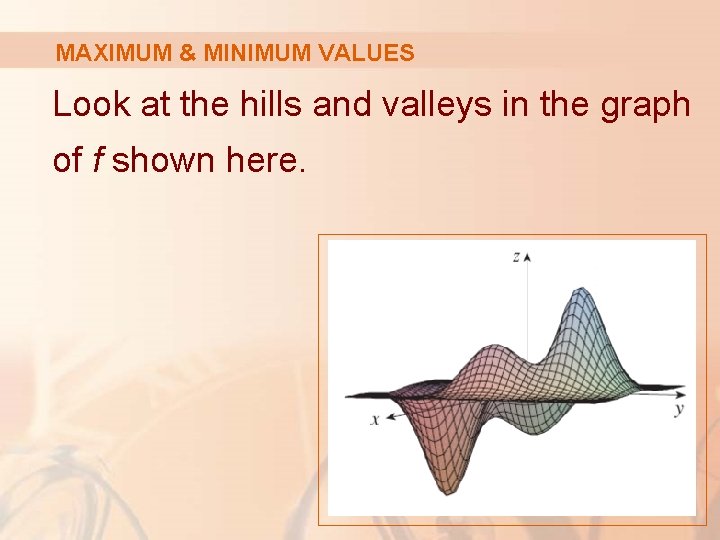
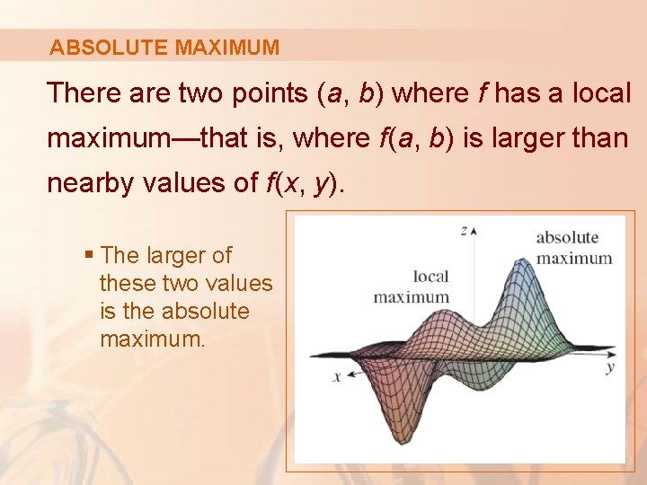
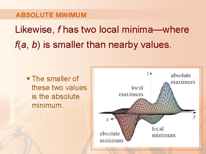
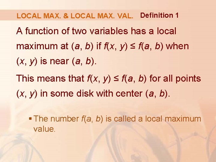
MAXIMUM & MINIMUM VALUES Look at the hills and valleys in the graph of f shown here.

ABSOLUTE MAXIMUM There are two points (a, b) where f has a local maximum—that is, where f(a, b) is larger than nearby values of f(x, y). § The larger of these two values is the absolute maximum.

ABSOLUTE MINIMUM Likewise, f has two local minima—where f(a, b) is smaller than nearby values. § The smaller of these two values is the absolute minimum.

LOCAL MAX. & LOCAL MAX. VAL. Definition 1 A function of two variables has a local maximum at (a, b) if f(x, y) ≤ f(a, b) when (x, y) is near (a, b). This means that f(x, y) ≤ f(a, b) for all points (x, y) in some disk with center (a, b). § The number f(a, b) is called a local maximum value.

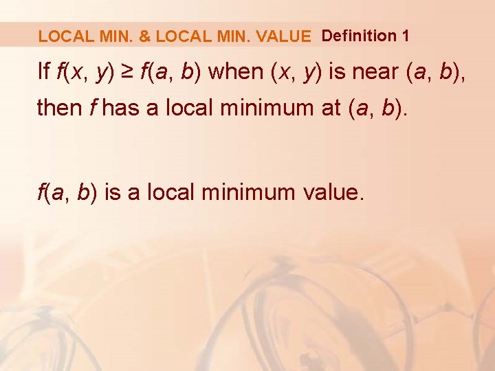
LOCAL MIN. & LOCAL MIN. VALUE Definition 1 If f(x, y) ≥ f(a, b) when (x, y) is near (a, b), then f has a local minimum at (a, b). f(a, b) is a local minimum value.

ABSOLUTE MAXIMUM & MINIMUM If the inequalities in Definition 1 hold for all points (x, y) in the domain of f, then f has an absolute maximum (or absolute minimum) at (a, b).

LOCAL MAXIMUM & MINIMUM Theorem 2 If f has a local maximum or minimum at (a, b) and the first-order partial derivatives of f exist there, then fx(a, b) = 0 and fy(a, b) = 0

LOCAL MAXIMUM & MINIMUM Proof Let g(x) = f(x, b). § If f has a local maximum (or minimum) at (a, b), then g has a local maximum (or minimum) at a. § So, g’(a) = 0 by Fermat’s Theorem.

LOCAL MAXIMUM & MINIMUM Proof However, g’(a) = fx(a, b) § See Equation 1 in Section 14. 3 § So, fx(a, b) = 0.

LOCAL MAXIMUM & MINIMUM Proof Similarly, by applying Fermat’s Theorem to the function G(y) = f(a, y), we obtain: fy(a, b) = 0

LOCAL MAXIMUM & MINIMUM If we put fx(a, b) = 0 and fy(a, b) = 0 in the equation of a tangent plane (Equation 2 in Section 14. 4), we get: z = z 0

THEOREM 2—GEOMETRIC INTERPRETATION Thus, the geometric interpretation of Theorem 2 is: § If the graph of f has a tangent plane at a local maximum or minimum, then the tangent plane must be horizontal.

CRITICAL POINT A point (a, b) is called a critical point (or stationary point) of f if either: § fx(a, b) = 0 and fy(a, b) = 0 § One of these partial derivatives does not exist.

CRITICAL POINTS Theorem 2 says that, if f has a local maximum or minimum at (a, b), then (a, b) is a critical point of f.

CRITICAL POINTS However, as in single-variable calculus, not all critical points give rise to maxima or minima. § At a critical point, a function could have a local maximum or a local minimum or neither.

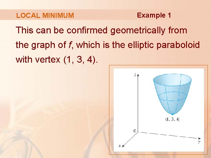
LOCAL MINIMUM Example 1 Let f(x, y) = x 2 + y 2 – 2 x – 6 y + 14 Then, fx(x, y) = 2 x – 2 fy(x, y) = 2 y – 6 § These partial derivatives are equal to 0 when x = 1 and y = 3. § So, the only critical point is (1, 3).

LOCAL MINIMUM Example 1 By completing the square, we find: f(x, y) = 4 + (x – 1)2 + (y – 3)2 § Since (x – 1)2 ≥ 0 and (y – 3)2 ≥ 0, we have f(x, y) ≥ 4 for all values of x and y. § So, f(1, 3) = 4 is a local minimum. § In fact, it is the absolute minimum of f.

LOCAL MINIMUM Example 1 This can be confirmed geometrically from the graph of f, which is the elliptic paraboloid with vertex (1, 3, 4).

EXTREME VALUES Example 2 Find the extreme values of f(x, y) = y 2 – x 2 § Since fx = – 2 x and fy = – 2 y, the only critical point is (0, 0).

EXTREME VALUES Example 2 Notice that, for points on the x-axis, we have y = 0. § So, f(x, y) = –x 2 < 0 (if x ≠ 0). For points on the y-axis, we have x = 0. § So, f(x, y) = y 2 > 0 (if y ≠ 0).

EXTREME VALUES Example 2 Thus, every disk with center (0, 0) contains points where f takes positive values as well as points where f takes negative values. § So, f(0, 0) = 0 can’t be an extreme value for f. § Hence, f has no extreme value.

MAXIMUM & MINIMUM VALUES Example 2 illustrates the fact that a function need not have a maximum or minimum value at a critical point.

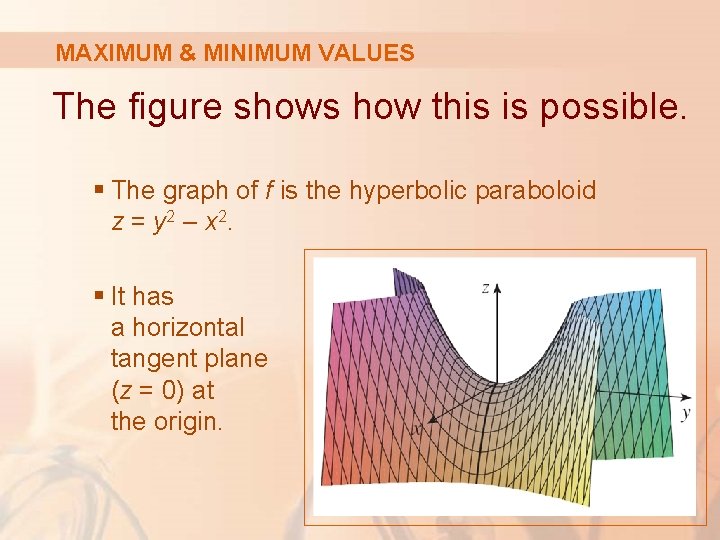
MAXIMUM & MINIMUM VALUES The figure shows how this is possible. § The graph of f is the hyperbolic paraboloid z = y 2 – x 2. § It has a horizontal tangent plane (z = 0) at the origin.

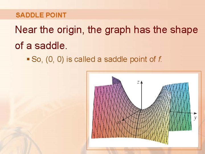
MAXIMUM & MINIMUM VALUES You can see that f(0, 0) = 0 is: § A maximum in the direction of the x-axis. § A minimum in the direction of the y-axis.

SADDLE POINT Near the origin, the graph has the shape of a saddle. § So, (0, 0) is called a saddle point of f.

EXTREME VALUE AT CRITICAL POINT We need to be able to determine whether or not a function has an extreme value at a critical point. The following test is analogous to the Second Derivative Test for functions of one variable.

SECOND DERIVATIVES TEST Theorem 3 Suppose that: § The second partial derivatives of f are continuous on a disk with center (a, b). § fx(a, b) = 0 and fy(a, b) = 0 [that is, (a, b) is a critical point of f].

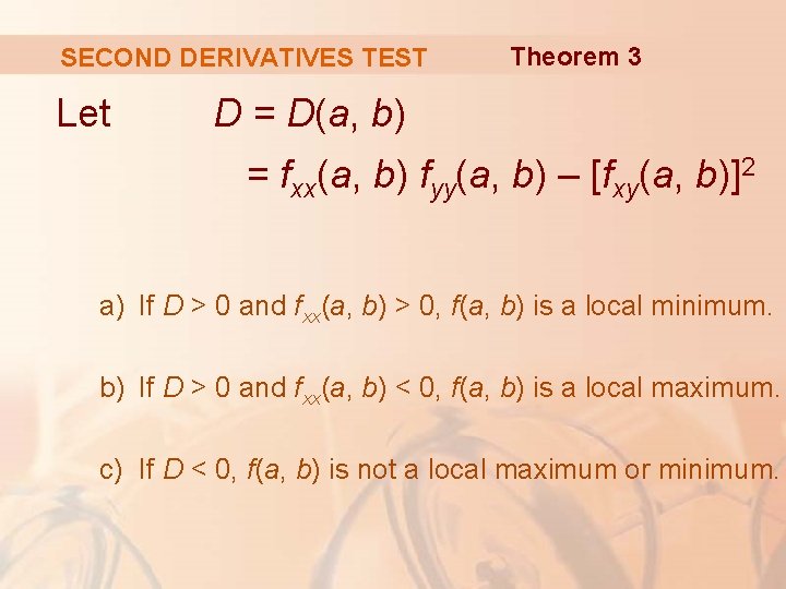
SECOND DERIVATIVES TEST Let Theorem 3 D = D(a, b) = fxx(a, b) fyy(a, b) – [fxy(a, b)]2 a) If D > 0 and fxx(a, b) > 0, f(a, b) is a local minimum. b) If D > 0 and fxx(a, b) < 0, f(a, b) is a local maximum. c) If D < 0, f(a, b) is not a local maximum or minimum.

SECOND DERIVATIVES TEST Note 1 In case c, § The point (a, b) is called a saddle point of f. § The graph of f crosses its tangent plane at (a, b).

SECOND DERIVATIVES TEST Note 2 If D = 0, the test gives no information: § f could have a local maximum or local minimum at (a, b), or (a, b) could be a saddle point of f.

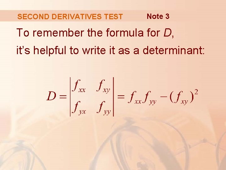
SECOND DERIVATIVES TEST Note 3 To remember the formula for D, it’s helpful to write it as a determinant:

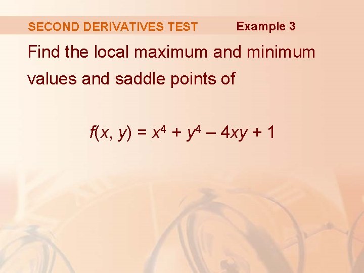
SECOND DERIVATIVES TEST Example 3 Find the local maximum and minimum values and saddle points of f(x, y) = x 4 + y 4 – 4 xy + 1

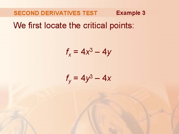
SECOND DERIVATIVES TEST Example 3 We first locate the critical points: fx = 4 x 3 – 4 y fy = 4 y 3 – 4 x

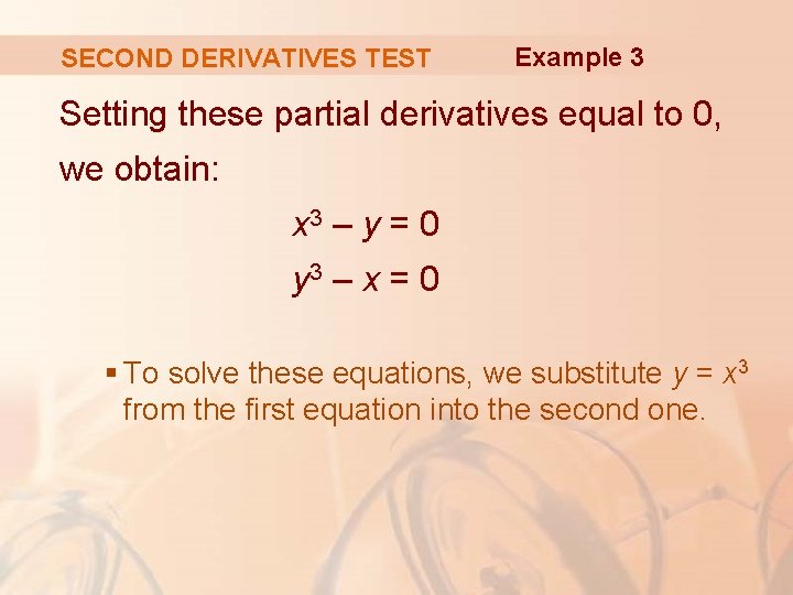
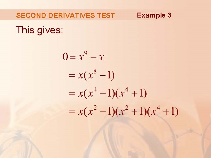
SECOND DERIVATIVES TEST Example 3 Setting these partial derivatives equal to 0, we obtain: x 3 – y = 0 y 3 – x = 0 § To solve these equations, we substitute y = x 3 from the first equation into the second one.

SECOND DERIVATIVES TEST This gives: Example 3

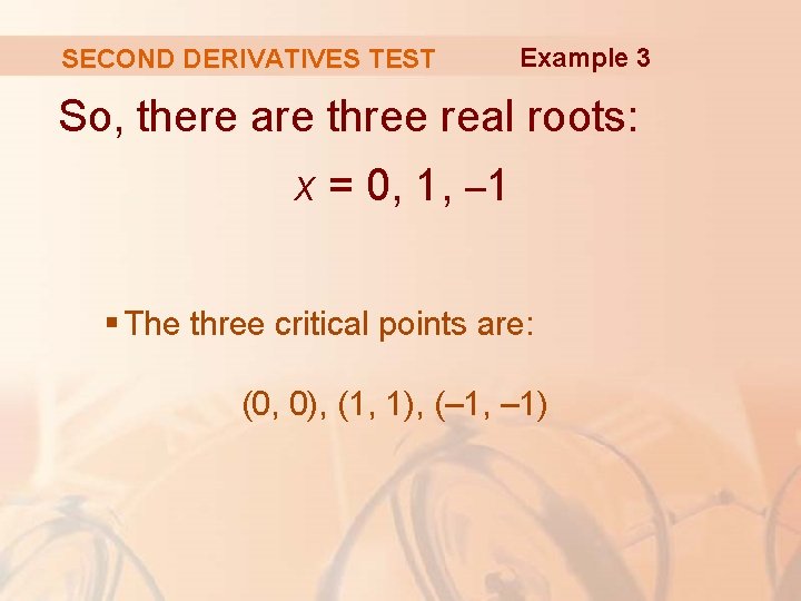
SECOND DERIVATIVES TEST Example 3 So, there are three real roots: x = 0, 1, – 1 § The three critical points are: (0, 0), (1, 1), (– 1, – 1)

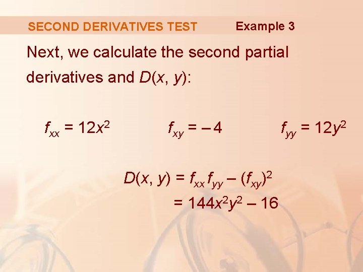
SECOND DERIVATIVES TEST Example 3 Next, we calculate the second partial derivatives and D(x, y): fxx = 12 x 2 fxy = – 4 D(x, y) = fxx fyy – (fxy)2 = 144 x 2 y 2 – 16 fyy = 12 y 2

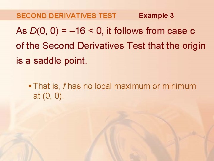
SECOND DERIVATIVES TEST Example 3 As D(0, 0) = – 16 < 0, it follows from case c of the Second Derivatives Test that the origin is a saddle point. § That is, f has no local maximum or minimum at (0, 0).

SECOND DERIVATIVES TEST Example 3 As D(1, 1) = 128 > 0 and fxx(1, 1) = 12 > 0, we see from case a of the test that f(1, 1) = – 1 is a local minimum. Similarly, we have D(– 1, – 1) = 128 > 0 and fxx(– 1, – 1) = 12 > 0. § So f(– 1, – 1) = – 1 is also a local minimum.

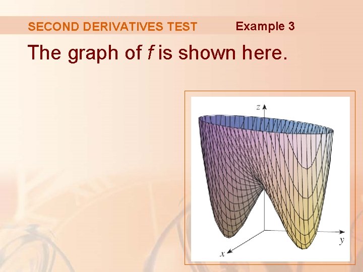
SECOND DERIVATIVES TEST Example 3 The graph of f is shown here.

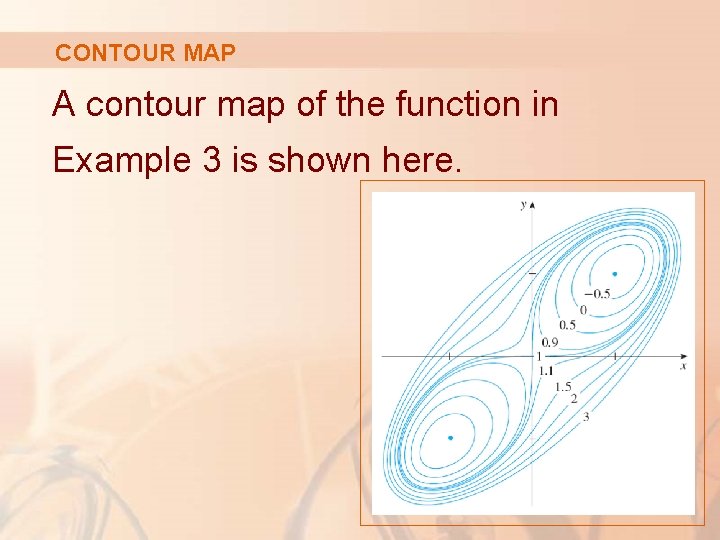
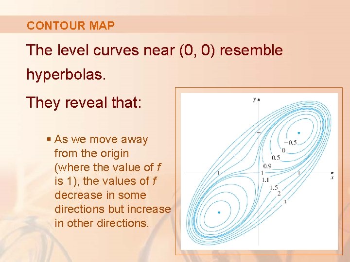
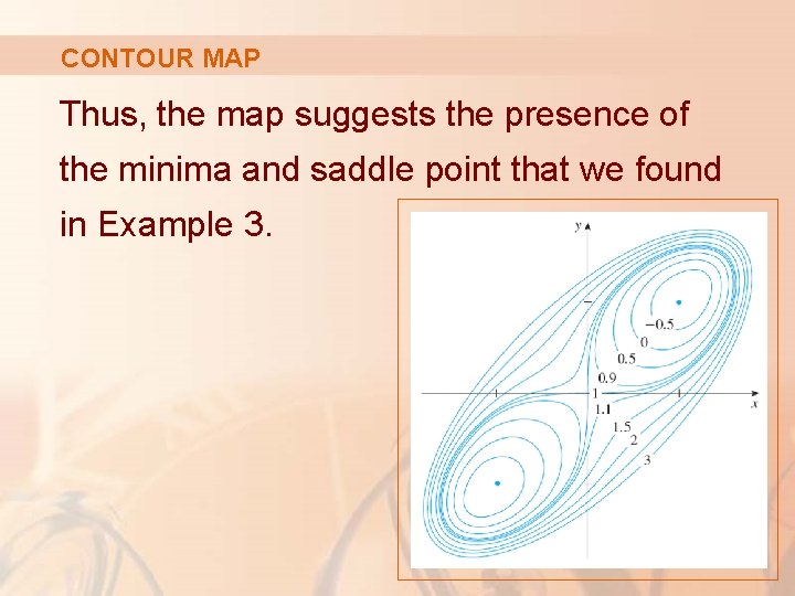
CONTOUR MAP A contour map of the function in Example 3 is shown here.

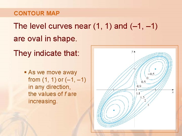
CONTOUR MAP The level curves near (1, 1) and (– 1, – 1) are oval in shape. They indicate that: § As we move away from (1, 1) or (– 1, – 1) in any direction, the values of f are increasing.

CONTOUR MAP The level curves near (0, 0) resemble hyperbolas. They reveal that: § As we move away from the origin (where the value of f is 1), the values of f decrease in some directions but increase in other directions.

CONTOUR MAP Thus, the map suggests the presence of the minima and saddle point that we found in Example 3.

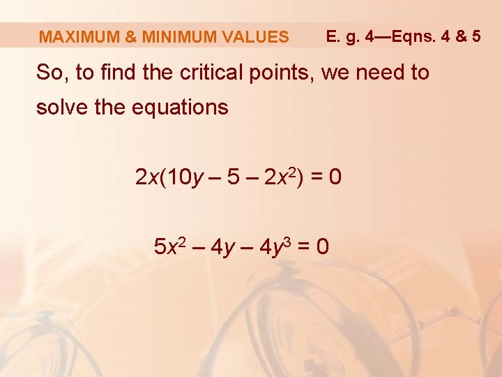
MAXIMUM & MINIMUM VALUES Example 4 Find and classify the critical points of the function f(x, y) = 10 x 2 y – 5 x 2 – 4 y 2 – x 4 – 2 y 4 Also, find the highest point on the graph of f.

MAXIMUM & MINIMUM VALUES Example 4 The first-order partial derivatives are: fx = 20 xy – 10 x – 4 x 3 fy = 10 x 2 – 8 y 3

MAXIMUM & MINIMUM VALUES E. g. 4—Eqns. 4 & 5 So, to find the critical points, we need to solve the equations 2 x(10 y – 5 – 2 x 2) = 0 5 x 2 – 4 y 3 = 0

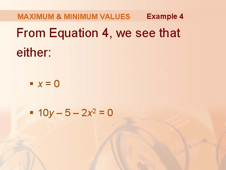
MAXIMUM & MINIMUM VALUES Example 4 From Equation 4, we see that either: § x=0 § 10 y – 5 – 2 x 2 = 0

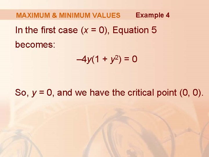
MAXIMUM & MINIMUM VALUES Example 4 In the first case (x = 0), Equation 5 becomes: – 4 y(1 + y 2) = 0 So, y = 0, and we have the critical point (0, 0).

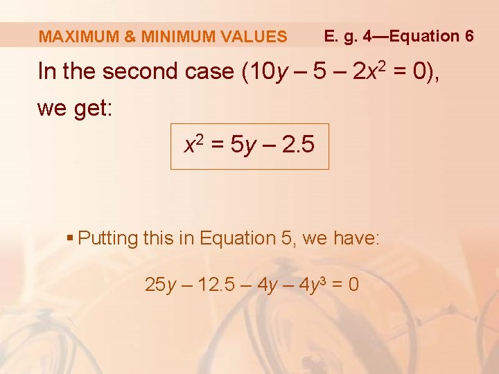
MAXIMUM & MINIMUM VALUES E. g. 4—Equation 6 In the second case (10 y – 5 – 2 x 2 = 0), we get: x 2 = 5 y – 2. 5 § Putting this in Equation 5, we have: 25 y – 12. 5 – 4 y 3 = 0

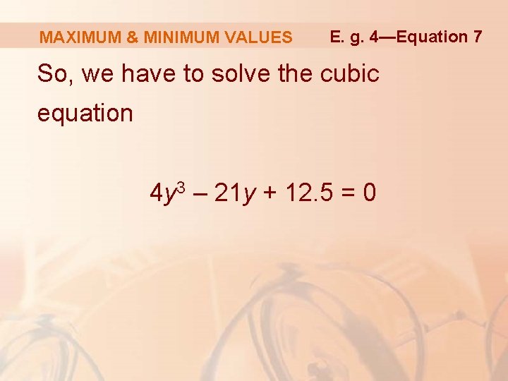
MAXIMUM & MINIMUM VALUES E. g. 4—Equation 7 So, we have to solve the cubic equation 4 y 3 – 21 y + 12. 5 = 0

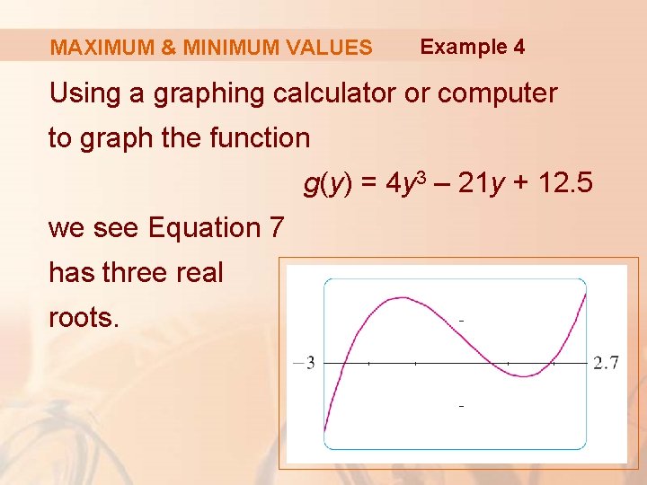
MAXIMUM & MINIMUM VALUES Example 4 Using a graphing calculator or computer to graph the function g(y) = 4 y 3 – 21 y + 12. 5 we see Equation 7 has three real roots.

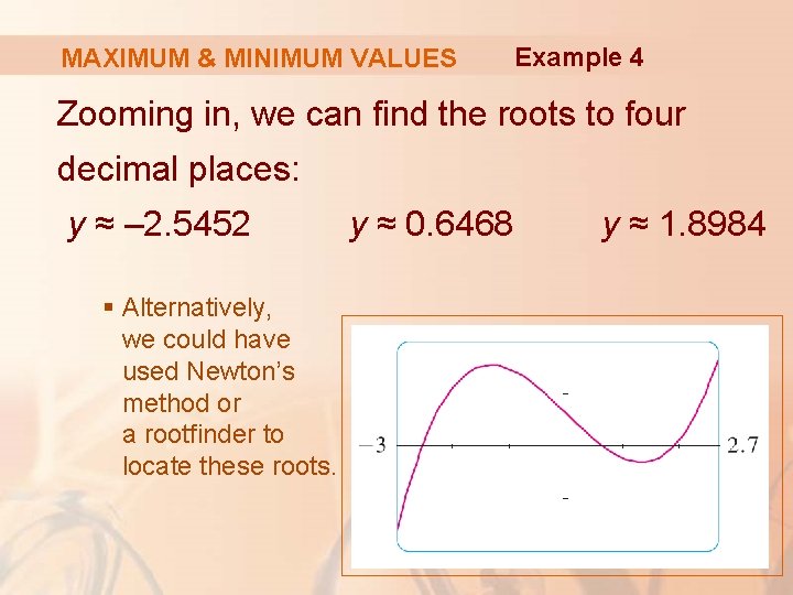
MAXIMUM & MINIMUM VALUES Example 4 Zooming in, we can find the roots to four decimal places: y ≈ – 2. 5452 § Alternatively, we could have used Newton’s method or a rootfinder to locate these roots. y ≈ 0. 6468 y ≈ 1. 8984

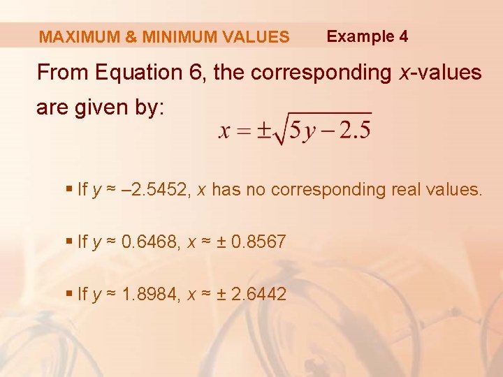
MAXIMUM & MINIMUM VALUES Example 4 From Equation 6, the corresponding x-values are given by: § If y ≈ – 2. 5452, x has no corresponding real values. § If y ≈ 0. 6468, x ≈ ± 0. 8567 § If y ≈ 1. 8984, x ≈ ± 2. 6442

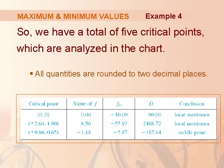
MAXIMUM & MINIMUM VALUES Example 4 So, we have a total of five critical points, which are analyzed in the chart. § All quantities are rounded to two decimal places.

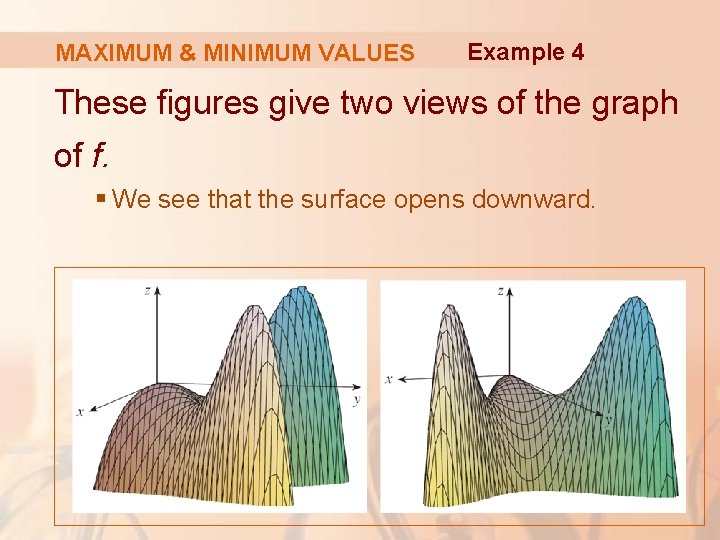
MAXIMUM & MINIMUM VALUES Example 4 These figures give two views of the graph of f. § We see that the surface opens downward.

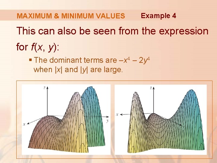
MAXIMUM & MINIMUM VALUES Example 4 This can also be seen from the expression for f(x, y): § The dominant terms are –x 4 – 2 y 4 when |x| and |y| are large.

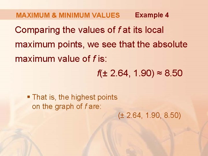
MAXIMUM & MINIMUM VALUES Example 4 Comparing the values of f at its local maximum points, we see that the absolute maximum value of f is: f(± 2. 64, 1. 90) ≈ 8. 50 § That is, the highest points on the graph of f are: (± 2. 64, 1. 90, 8. 50)

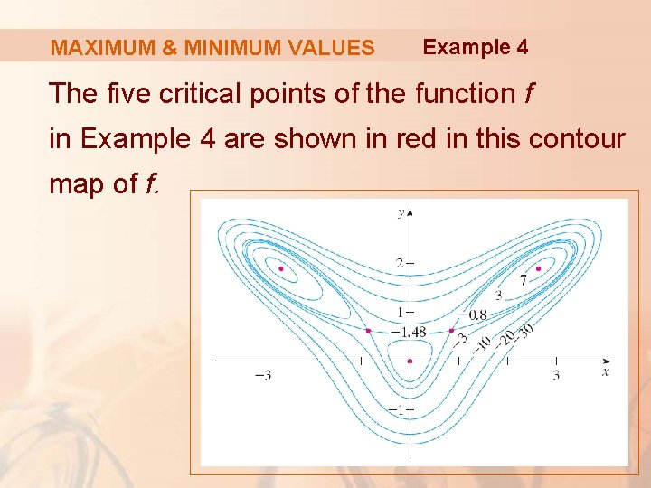
MAXIMUM & MINIMUM VALUES Example 4 The five critical points of the function f in Example 4 are shown in red in this contour map of f.

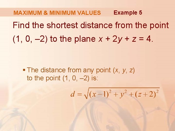
MAXIMUM & MINIMUM VALUES Example 5 Find the shortest distance from the point (1, 0, – 2) to the plane x + 2 y + z = 4. § The distance from any point (x, y, z) to the point (1, 0, – 2) is:

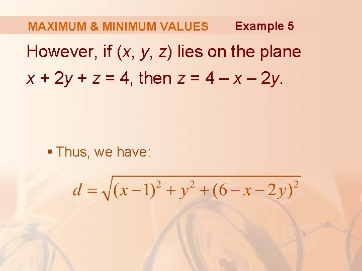
MAXIMUM & MINIMUM VALUES Example 5 However, if (x, y, z) lies on the plane x + 2 y + z = 4, then z = 4 – x – 2 y. § Thus, we have:

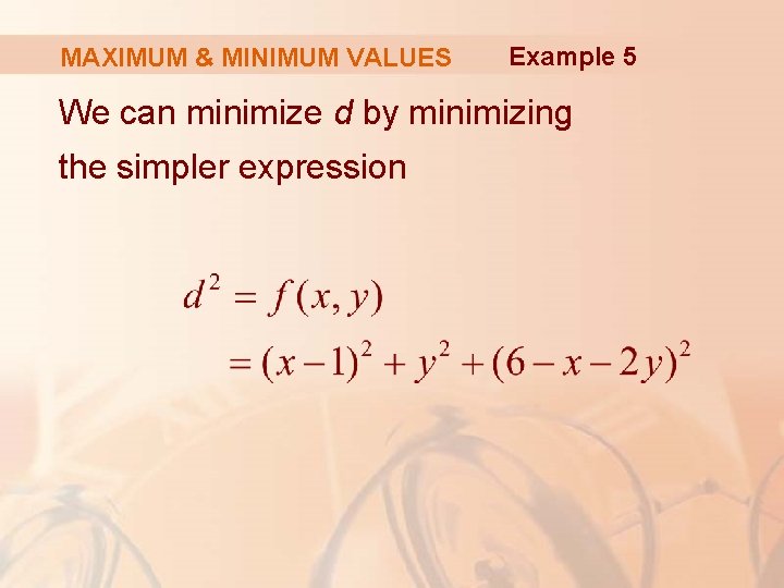
MAXIMUM & MINIMUM VALUES Example 5 We can minimize d by minimizing the simpler expression

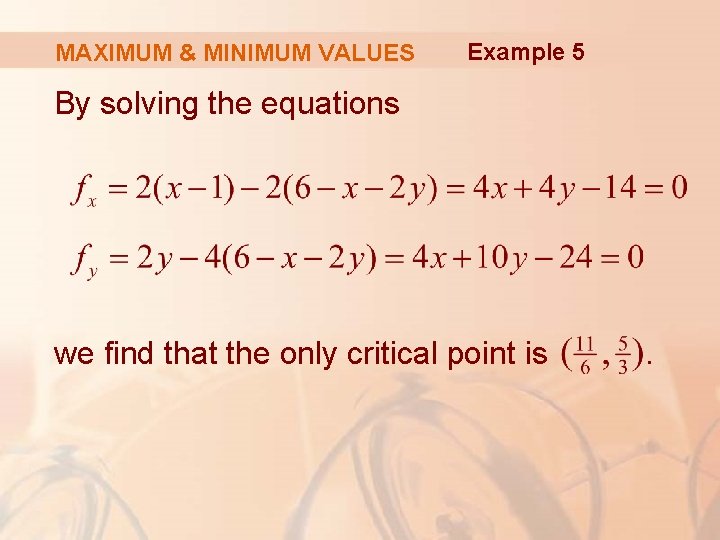
MAXIMUM & MINIMUM VALUES Example 5 By solving the equations we find that the only critical point is .

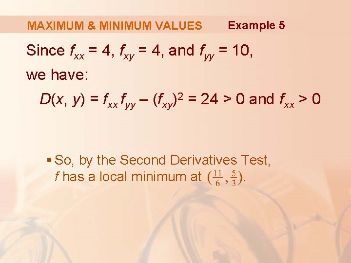
MAXIMUM & MINIMUM VALUES Example 5 Since fxx = 4, fxy = 4, and fyy = 10, we have: D(x, y) = fxx fyy – (fxy)2 = 24 > 0 and fxx > 0 § So, by the Second Derivatives Test, f has a local minimum at.

MAXIMUM & MINIMUM VALUES Example 5 Intuitively, we can see that this local minimum is actually an absolute minimum: § There must be a point on the given plane that is closest to (1, 0, – 2).

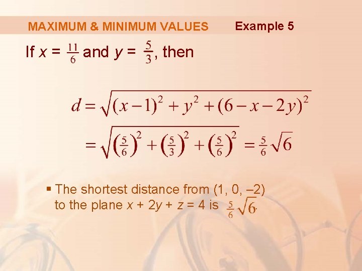
MAXIMUM & MINIMUM VALUES If x = and y = Example 5 , then § The shortest distance from (1, 0, – 2) to the plane x + 2 y + z = 4 is.

MAXIMUM & MINIMUM VALUES Example 6 A rectangular box without a lid is to be made from 12 m 2 of cardboard. Find the maximum volume of such a box.

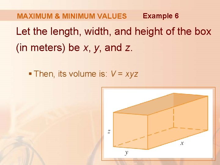
MAXIMUM & MINIMUM VALUES Example 6 Let the length, width, and height of the box (in meters) be x, y, and z. § Then, its volume is: V = xyz

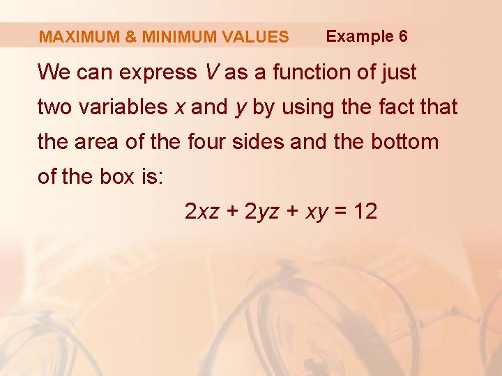
MAXIMUM & MINIMUM VALUES Example 6 We can express V as a function of just two variables x and y by using the fact that the area of the four sides and the bottom of the box is: 2 xz + 2 yz + xy = 12

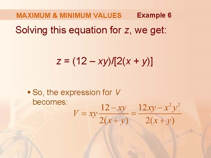
MAXIMUM & MINIMUM VALUES Example 6 Solving this equation for z, we get: z = (12 – xy)/[2(x + y)] § So, the expression for V becomes:

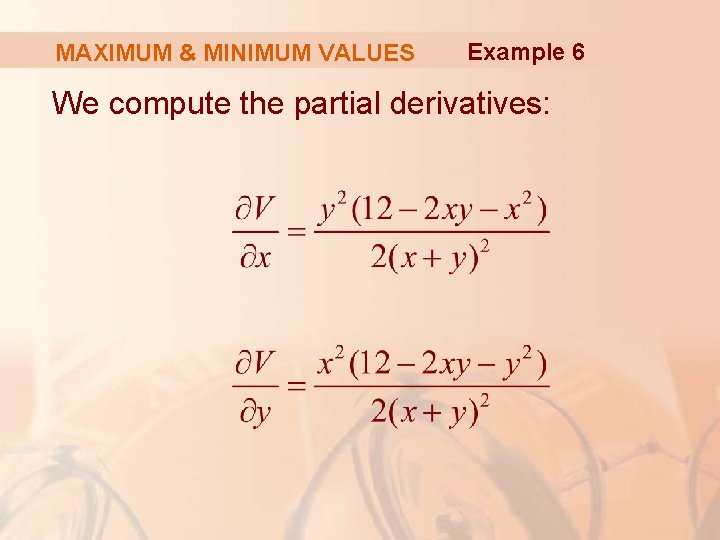
MAXIMUM & MINIMUM VALUES Example 6 We compute the partial derivatives:

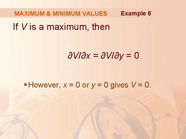
MAXIMUM & MINIMUM VALUES Example 6 If V is a maximum, then ∂V/∂x = ∂V/∂y = 0 § However, x = 0 or y = 0 gives V = 0.

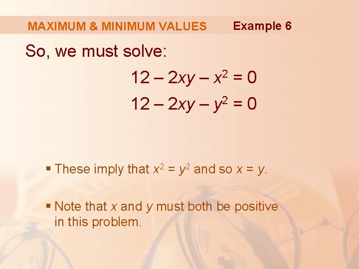
MAXIMUM & MINIMUM VALUES Example 6 So, we must solve: 12 – 2 xy – x 2 = 0 12 – 2 xy – y 2 = 0 § These imply that x 2 = y 2 and so x = y. § Note that x and y must both be positive in this problem.

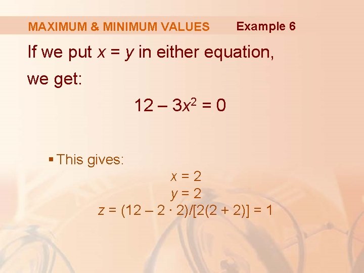
MAXIMUM & MINIMUM VALUES Example 6 If we put x = y in either equation, we get: 12 – 3 x 2 = 0 § This gives: x=2 y=2 z = (12 – 2 ∙ 2)/[2(2 + 2)] = 1

MAXIMUM & MINIMUM VALUES Example 6 We could use the Second Derivatives Test to show that this gives a local maximum of V.

MAXIMUM & MINIMUM VALUES Example 6 Alternatively, we could simply argue from the physical nature of this problem that there must be an absolute maximum volume, which has to occur at a critical point of V. § So, it must occur when x = 2, y = 2, z = 1.

MAXIMUM & MINIMUM VALUES Example 6 Then, V=2∙ 2∙ 1 =4 § Thus, the maximum volume of the box is 4 m 3.

ABSOLUTE MAXIMUM & MINIMUM VALUES For a function f of one variable, the Extreme Value Theorem says that: § If f is continuous on a closed interval [a, b], then f has an absolute minimum value and an absolute maximum value.

ABSOLUTE MAXIMUM & MINIMUM VALUES According to the Closed Interval Method in Section 4. 1, we found these by evaluating f at both: § The critical numbers § The endpoints a and b

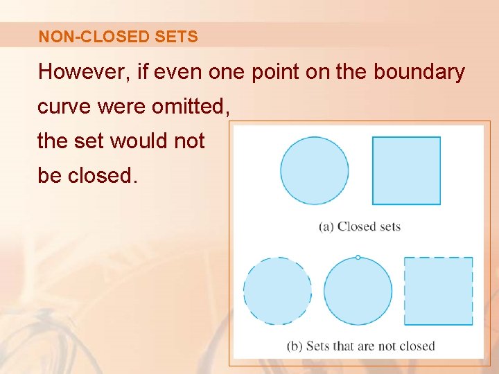
CLOSED SET There is a similar situation for functions of two variables. Just as a closed interval contains its endpoints, a closed set in is one that contains all its boundary points.

BOUNDARY POINT A boundary point of D is a point (a, b) such that every disk with center (a, b) contains points in D and also points not in D.

CLOSED SETS For instance, the disk D = {(x, y) | x 2 + y 2 ≤ 1} which consists of all points on and inside the circle x 2 + y 2 = 1 is a closed set because: § It contains all of its boundary points (the points on the circle x 2 + y 2 = 1).

NON-CLOSED SETS However, if even one point on the boundary curve were omitted, the set would not be closed.

BOUNDED SET A bounded set in is one that is contained within some disk. § In other words, it is finite in extent.

CLOSED & BOUNDED SETS Then, in terms of closed and bounded sets, we can state the following counterpart of the Extreme Value Theorem (EVT) for functions of two variables in two dimensions.

EVT (TWO-VARIABLE FUNCTIONS) Theorem 8 If f is continuous on a closed, bounded set D in , then f attains an absolute maximum value f(x 1, y 1) and an absolute minimum value f(x 2, y 2) at some points (x 1, y 1) and (x 2, y 2) in D.

EVT (TWO-VARIABLE FUNCTIONS) To find the extreme values guaranteed by Theorem 8, we note that, by Theorem 2, if f has an extreme value at (x 1, y 1), then (x 1, y 1) is either: § A critical point of f § A boundary point of D

EVT (TWO-VARIABLE FUNCTIONS) Thus, we have the following extension of the Closed Interval Method.

CLOSED INTVL. METHOD (EXTN. ) Method 9 To find the absolute maximum and minimum values of a continuous function f on a closed, bounded set D: 1. Find the values of f at the critical points of f in D. 2. Find the extreme values of f on the boundary of D. 3. The largest value from steps 1 and 2 is the absolute maximum value. The smallest is the absolute minimum value.

CLOSED & BOUNDED SETS Example 7 Find the absolute maximum and minimum values of the function f(x, y) = x 2 – 2 xy + 2 y on the rectangle D = {(x, y) | 0 ≤ x ≤ 3, 0 ≤ y ≤ 2}

CLOSED & BOUNDED SETS Example 7 As f is a polynomial, it is continuous on the closed, bounded rectangle D. § So, Theorem 8 tells us there is both an absolute maximum and an absolute minimum.

CLOSED & BOUNDED SETS Example 7 According to step 1 in Method 9, we first find the critical points. § These occur when fx = 2 x – 2 y = 0 fy = – 2 x + 2 = 0 § So, the only critical point is (1, 1). § The value of f there is f(1, 1) = 1.

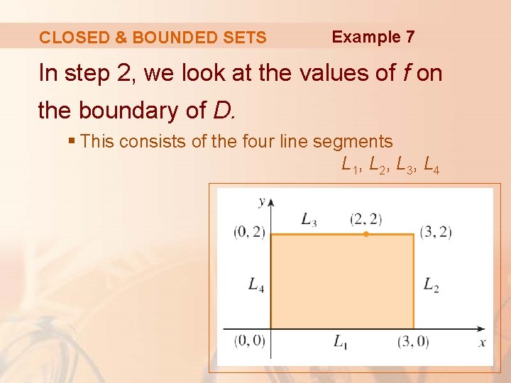
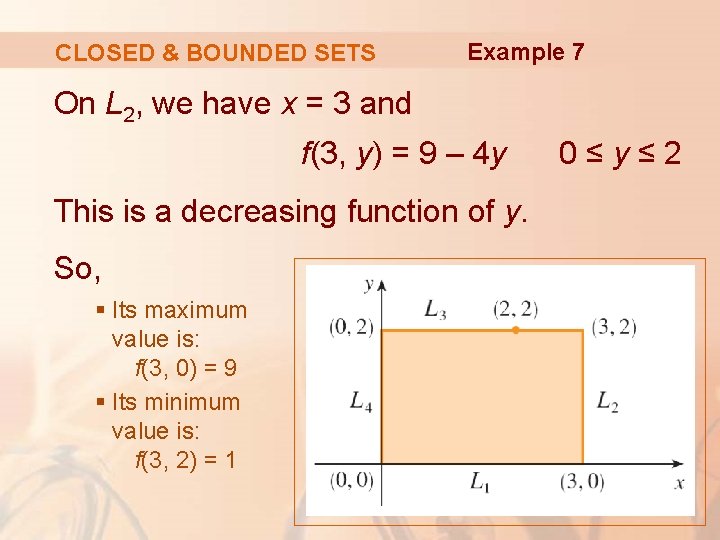
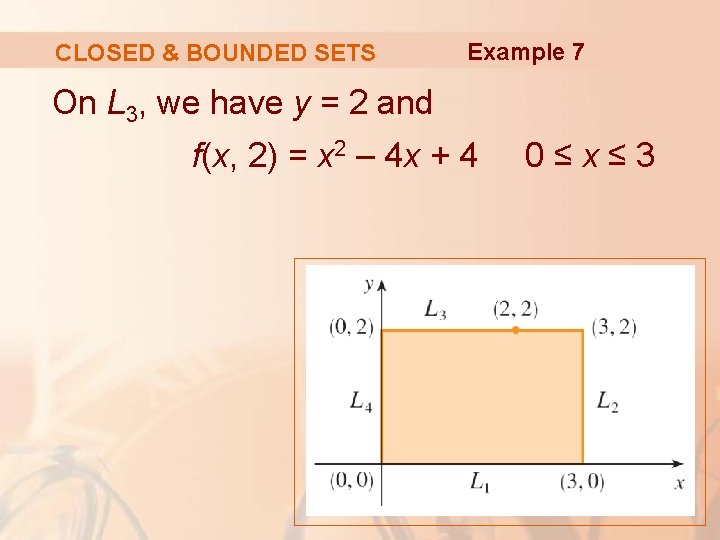
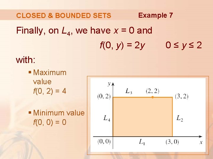
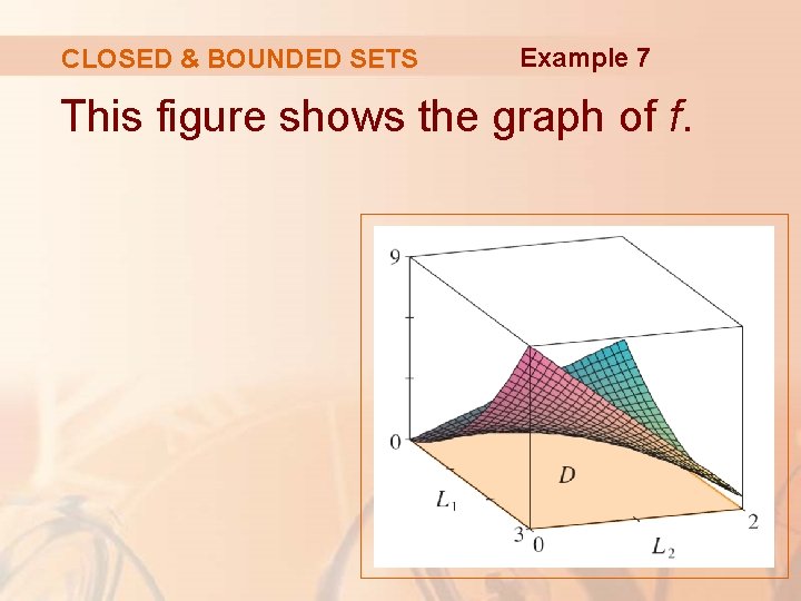
CLOSED & BOUNDED SETS Example 7 In step 2, we look at the values of f on the boundary of D. § This consists of the four line segments L 1, L 2, L 3, L 4

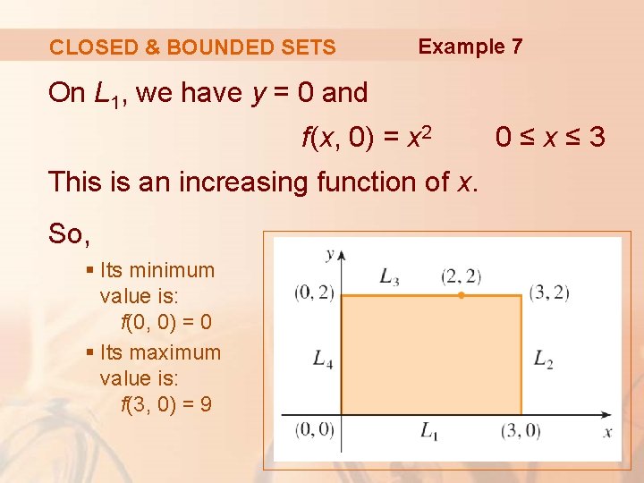
CLOSED & BOUNDED SETS Example 7 On L 1, we have y = 0 and f(x, 0) = x 2 This is an increasing function of x. So, § Its minimum value is: f(0, 0) = 0 § Its maximum value is: f(3, 0) = 9 0≤x≤ 3

CLOSED & BOUNDED SETS Example 7 On L 2, we have x = 3 and f(3, y) = 9 – 4 y This is a decreasing function of y. So, § Its maximum value is: f(3, 0) = 9 § Its minimum value is: f(3, 2) = 1 0≤y≤ 2

CLOSED & BOUNDED SETS Example 7 On L 3, we have y = 2 and f(x, 2) = x 2 – 4 x + 4 0≤x≤ 3

CLOSED & BOUNDED SETS Example 7 By the methods of Chapter 4, or simply by observing that f(x, 2) = (x – 2)2, we see that: § The minimum value of the function is f(2, 2) = 0. § The maximum value of the function is f(0, 2) = 4.

CLOSED & BOUNDED SETS Example 7 Finally, on L 4, we have x = 0 and f(0, y) = 2 y with: § Maximum value f(0, 2) = 4 § Minimum value f(0, 0) = 0 0≤y≤ 2

CLOSED & BOUNDED SETS Example 7 Thus, on the boundary, § The minimum value of f is 0. § The maximum value of f is 9.

CLOSED & BOUNDED SETS Example 7 In step 3, we compare these values with the value f(1, 1) = 1 at the critical point. We conclude that: § The absolute maximum value of f on D is f(3, 0) = 9. § The absolute minimum value of f on D is f(0, 0) = f(2, 2) = 0.

CLOSED & BOUNDED SETS Example 7 This figure shows the graph of f.

SECOND DERIVATIVES TEST We close this section by giving a proof of the first part of the Second Derivatives Test. § The second part has a similar proof.

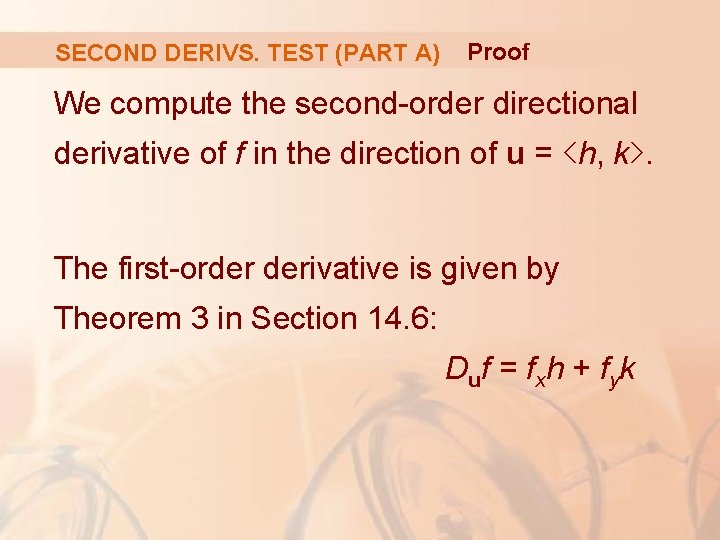
SECOND DERIVS. TEST (PART A) Proof We compute the second-order directional derivative of f in the direction of u = <h, k>. The first-order derivative is given by Theorem 3 in Section 14. 6: Duf = fxh + fyk

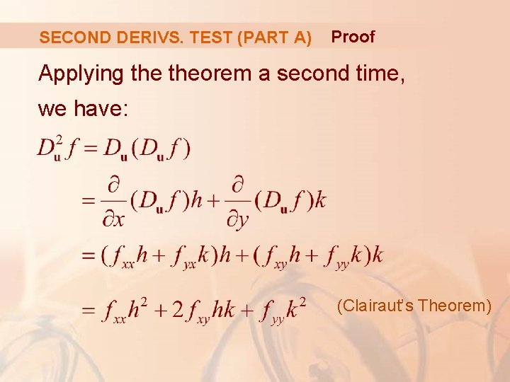
SECOND DERIVS. TEST (PART A) Proof Applying theorem a second time, we have: (Clairaut’s Theorem)

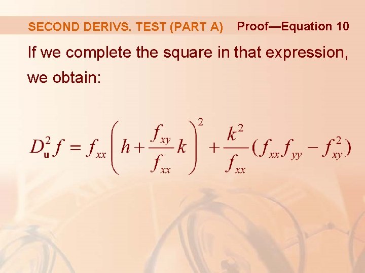
SECOND DERIVS. TEST (PART A) Proof—Equation 10 If we complete the square in that expression, we obtain:

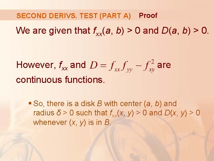
SECOND DERIVS. TEST (PART A) Proof We are given that fxx(a, b) > 0 and D(a, b) > 0. However, fxx and are continuous functions. § So, there is a disk B with center (a, b) and radius δ > 0 such that fxx(x, y) > 0 and D(x, y) > 0 whenever (x, y) is in B.

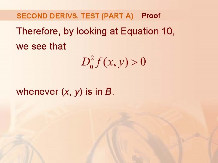
SECOND DERIVS. TEST (PART A) Proof Therefore, by looking at Equation 10, we see that whenever (x, y) is in B.

SECOND DERIVS. TEST (PART A) Proof This means that: § If C is the curve obtained by intersecting the graph of f with the vertical plane through P(a, b, f(a, b)) in the direction of u, then C is concave upward on an interval of length 2δ.

SECOND DERIVS. TEST (PART A) Proof This is true in the direction of every vector u. § So, if we restrict (x, y) to lie in B, the graph of f lies above its horizontal tangent plane at P.

SECOND DERIVS. TEST (PART A) Proof Thus, f(x, y) ≥ f(a, b) whenever (x, y) is in B. § This shows that f(a, b) is a local minimum.