15 MULTIPLE INTEGRALS MULTIPLE INTEGRALS 15 9 Change

15 MULTIPLE INTEGRALS

MULTIPLE INTEGRALS 15. 9 Change of Variables in Multiple Integrals In this section, we will learn about: The change of variables in double and triple integrals.

CHANGE OF VARIABLES IN SINGLE INTEGRALS In one-dimensional calculus. we often use a change of variable (a substitution) to simplify an integral.

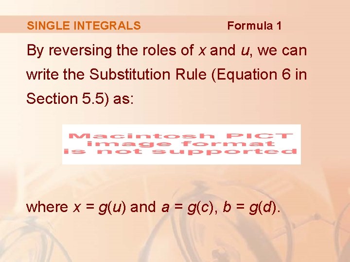
SINGLE INTEGRALS Formula 1 By reversing the roles of x and u, we can write the Substitution Rule (Equation 6 in Section 5. 5) as: where x = g(u) and a = g(c), b = g(d).

SINGLE INTEGRALS Formula 2 Another way of writing Formula 1 is as follows:

CHANGE OF VARIABLES IN DOUBLE INTEGRALS A change of variables can also be useful in double integrals. § We have already seen one example of this: conversion to polar coordinates.

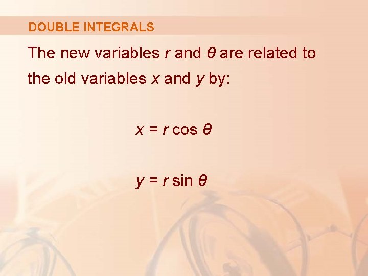
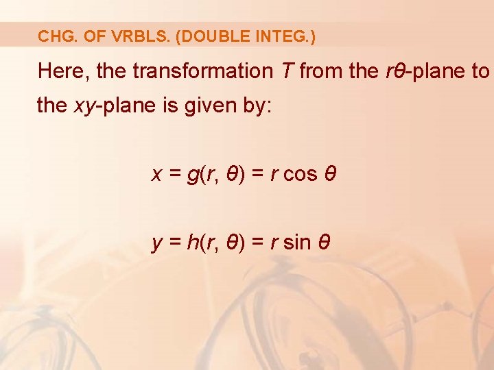
DOUBLE INTEGRALS The new variables r and θ are related to the old variables x and y by: x = r cos θ y = r sin θ

DOUBLE INTEGRALS The change of variables formula (Formula 2 in Section 15. 4) can be written as: where S is the region in the rθ-plane that corresponds to the region R in the xy-plane.

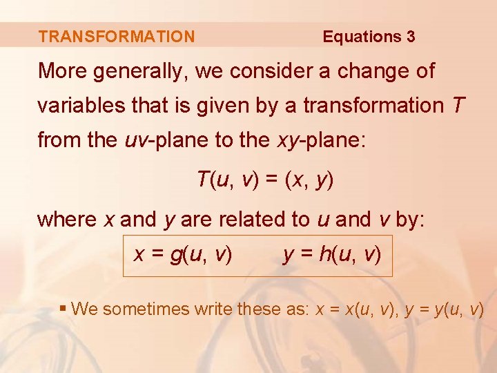
Equations 3 TRANSFORMATION More generally, we consider a change of variables that is given by a transformation T from the uv-plane to the xy-plane: T(u, v) = (x, y) where x and y are related to u and v by: x = g(u, v) y = h(u, v) § We sometimes write these as: x = x(u, v), y = y(u, v)

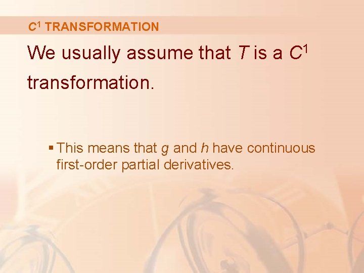
C 1 TRANSFORMATION We usually assume that T is a C 1 transformation. § This means that g and h have continuous first-order partial derivatives.

TRANSFORMATION A transformation T is really just a function whose domain and range are both subsets of .

IMAGE & ONE-TO-ONE TRANSFORMATION If T(u 1, v 1) = (x 1, y 1), then the point (x 1, y 1) is called the image of the point (u 1, v 1). If no two points have the same image, T is called one-to-one.

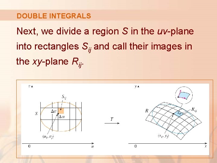
CHANGE OF VARIABLES The figure shows the effect of a transformation T on a region S in the uv-plane. § T transforms S into a region R in the xy-plane called the image of S, consisting of the images of all points in S.

INVERSE TRANSFORMATION If T is a one-to-one transformation, it has an inverse transformation T– 1 from the xy–plane to the uv-plane.

INVERSE TRANSFORMATION Then, it may be possible to solve Equations 3 for u and v in terms of x and y : u = G(x, y) v = H(x, y)

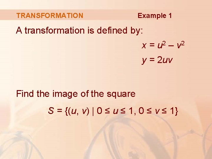
TRANSFORMATION Example 1 A transformation is defined by: x = u 2 – v 2 y = 2 uv Find the image of the square S = {(u, v) | 0 ≤ u ≤ 1, 0 ≤ v ≤ 1}

TRANSFORMATION Example 1 The transformation maps the boundary of S into the boundary of the image. § So, we begin by finding the images of the sides of S.

TRANSFORMATION Example 1 The first side, S 1, is given by: v = 0 (0 ≤ u ≤ 1)

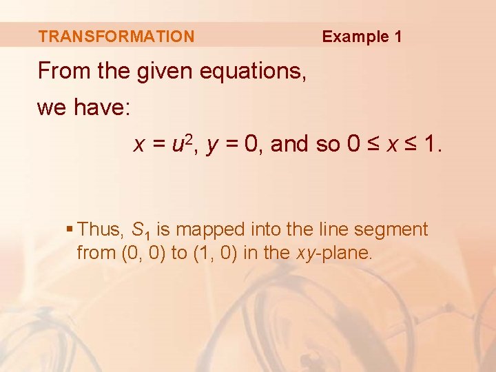
TRANSFORMATION Example 1 From the given equations, we have: x = u 2, y = 0, and so 0 ≤ x ≤ 1. § Thus, S 1 is mapped into the line segment from (0, 0) to (1, 0) in the xy-plane.

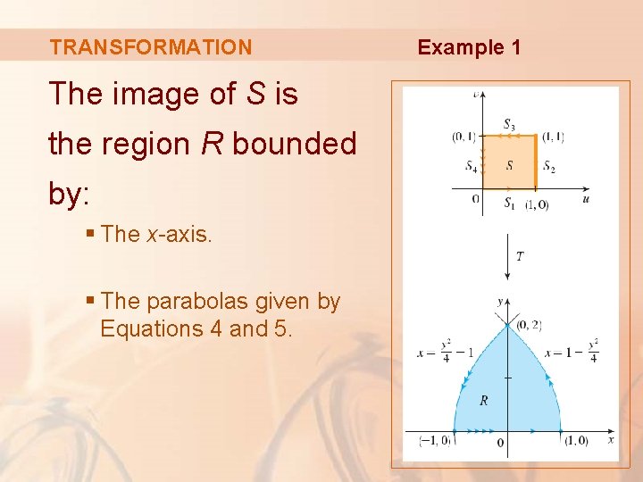
E. g. 1—Equation 4 TRANSFORMATION The second side, S 2, is: u = 1 (0 ≤ v ≤ 1) § Putting u = 1 in the given equations, we get: x = 1 – v 2 y = 2 v

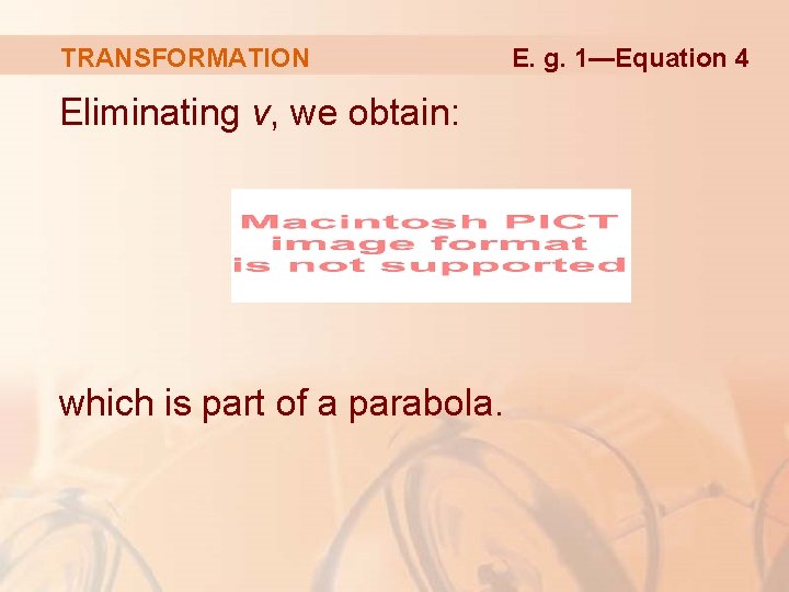
TRANSFORMATION Eliminating v, we obtain: which is part of a parabola. E. g. 1—Equation 4

TRANSFORMATION E. g. 1—Equation 5 Similarly, S 3 is given by: v = 1 (0 ≤ u ≤ 1) Its image is the parabolic arc

TRANSFORMATION Example 1 Finally, S 4 is given by: u = 0(0 ≤ v ≤ 1) Its image is: x = –v 2, y = 0 that is, – 1 ≤ x ≤ 0

TRANSFORMATION Example 1 Notice that as, we move around the square in the counterclockwise direction, we also move around the parabolic region in the counterclockwise direction.

TRANSFORMATION The image of S is the region R bounded by: § The x-axis. § The parabolas given by Equations 4 and 5. Example 1

DOUBLE INTEGRALS Now, let’s see how a change of variables affects a double integral.

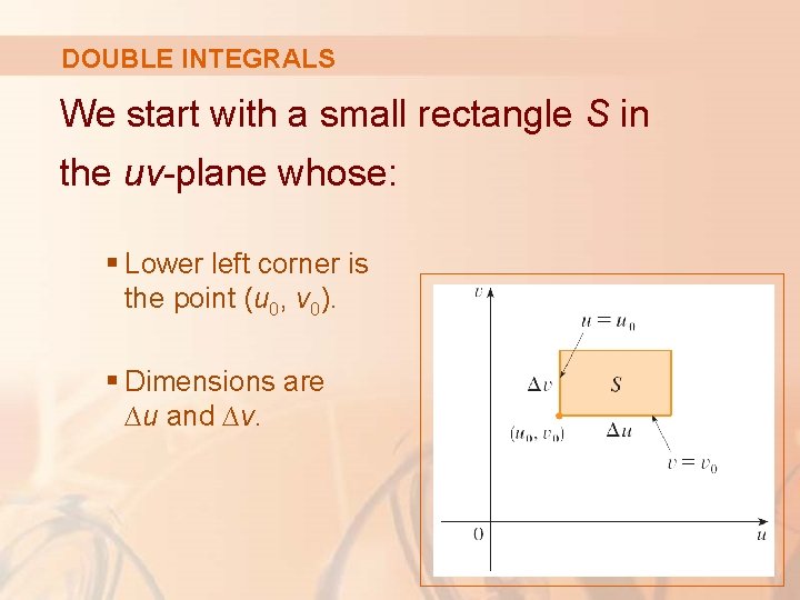
DOUBLE INTEGRALS We start with a small rectangle S in the uv-plane whose: § Lower left corner is the point (u 0, v 0). § Dimensions are ∆u and ∆v.

DOUBLE INTEGRALS The image of S is a region R in the xy-plane, one of whose boundary points is: (x 0, y 0) = T(u 0, v 0)

DOUBLE INTEGRALS The vector r(u, v) = g(u, v) i + h(u, v) j is the position vector of the image of the point (u, v).

DOUBLE INTEGRALS The equation of the lower side of S is: v = v 0 § Its image curve is given by the vector function r(u, v 0).

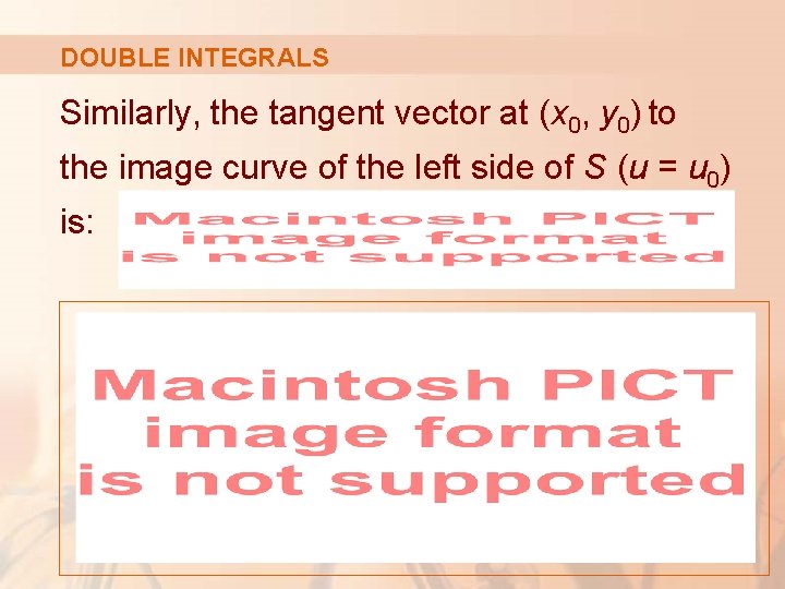
DOUBLE INTEGRALS The tangent vector at (x 0, y 0) to this image curve is:

DOUBLE INTEGRALS Similarly, the tangent vector at (x 0, y 0) to the image curve of the left side of S (u = u 0) is:

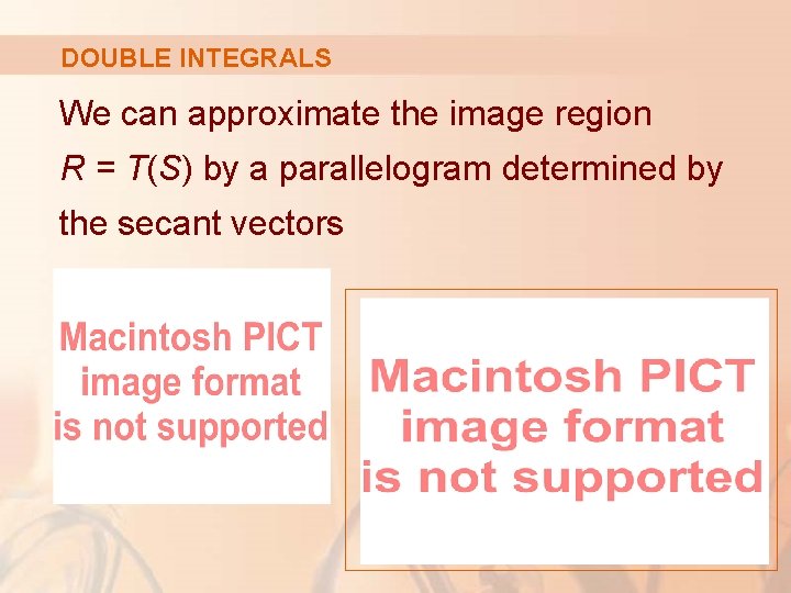
DOUBLE INTEGRALS We can approximate the image region R = T(S) by a parallelogram determined by the secant vectors

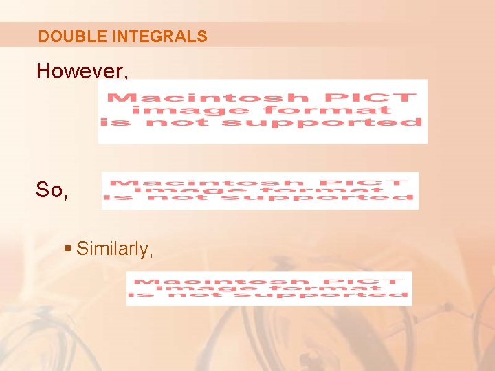
DOUBLE INTEGRALS However, So, § Similarly,

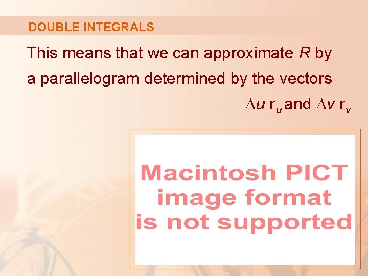
DOUBLE INTEGRALS This means that we can approximate R by a parallelogram determined by the vectors ∆u ru and ∆v rv

DOUBLE INTEGRALS Equation 6 Thus, we can approximate the area of R by the area of this parallelogram, which, from Section 12. 4, is: |(∆u ru) x (∆v rv)| = |ru x rv| ∆u ∆v

DOUBLE INTEGRALS Computing the cross product, we obtain:

JACOBIAN The determinant that arises in this calculation is called the Jacobian of the transformation. § It is given a special notation.

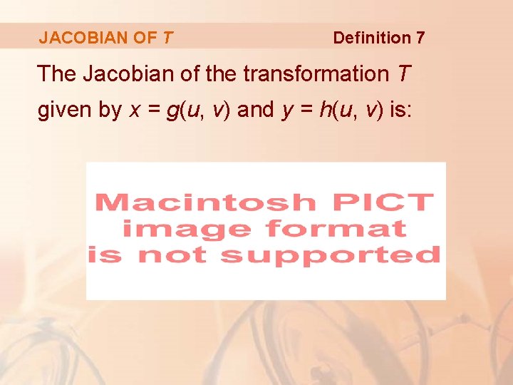
JACOBIAN OF T Definition 7 The Jacobian of the transformation T given by x = g(u, v) and y = h(u, v) is:

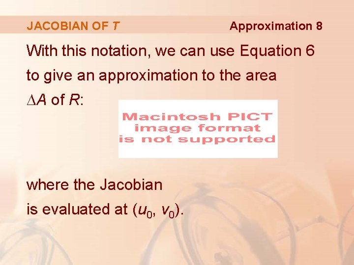
JACOBIAN OF T Approximation 8 With this notation, we can use Equation 6 to give an approximation to the area ∆A of R: where the Jacobian is evaluated at (u 0, v 0).

JACOBIAN The Jacobian is named after the German mathematician Carl Gustav Jacobi (1804– 1851). § The French mathematician Cauchy first used these special determinants involving partial derivatives. § Jacobi, though, developed them into a method for evaluating multiple integrals.

DOUBLE INTEGRALS Next, we divide a region S in the uv-plane into rectangles Sij and call their images in the xy-plane Rij.

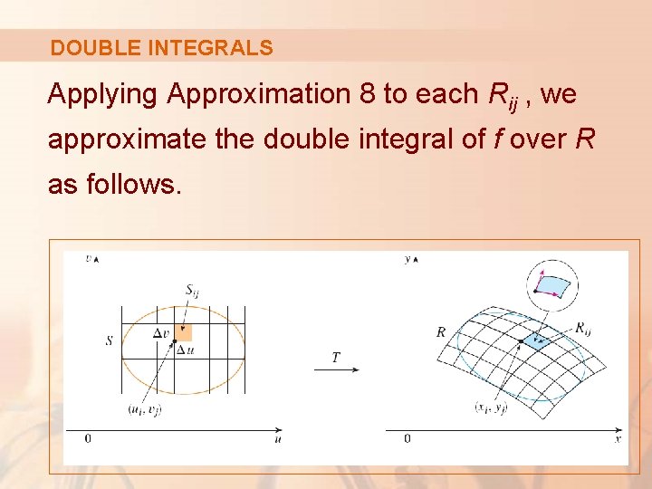
DOUBLE INTEGRALS Applying Approximation 8 to each Rij , we approximate the double integral of f over R as follows.

DOUBLE INTEGRALS where the Jacobian is evaluated at (ui, vj).

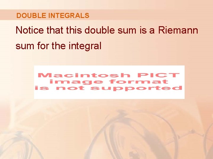
DOUBLE INTEGRALS Notice that this double sum is a Riemann sum for the integral

DOUBLE INTEGRALS The foregoing argument suggests that the following theorem is true. § A full proof is given in books on advanced calculus.

CHG. OF VRBLS. (DOUBLE INTEG. ) Theorem 9 Suppose: § T is a C 1 transformation whose Jacobian is nonzero and that maps a region S in the uv-plane onto a region R in the xy-plane. § f is continuous on R and that R and S are type I or type II plane regions. § T is one-to-one, except perhaps on the boundary of S.

CHG. OF VRBLS. (DOUBLE INTEG. ) Theorem 9 Then,

CHG. OF VRBLS. (DOUBLE INTEG. ) Theorem 9 says that we change from an integral in x and y to an integral in u and v by expressing x and y in terms of u and v and writing:

CHG. OF VRBLS. (DOUBLE INTEG. ) Notice the similarity between Theorem 9 and the one-dimensional formula in Equation 2. § Instead of the derivative dx/du, we have the absolute value of the Jacobian, that is, |∂(x, y)/∂(u, v)|

CHG. OF VRBLS. (DOUBLE INTEG. ) As a first illustration of Theorem 9, we show that the formula for integration in polar coordinates is just a special case.

CHG. OF VRBLS. (DOUBLE INTEG. ) Here, the transformation T from the rθ-plane to the xy-plane is given by: x = g(r, θ) = r cos θ y = h(r, θ) = r sin θ

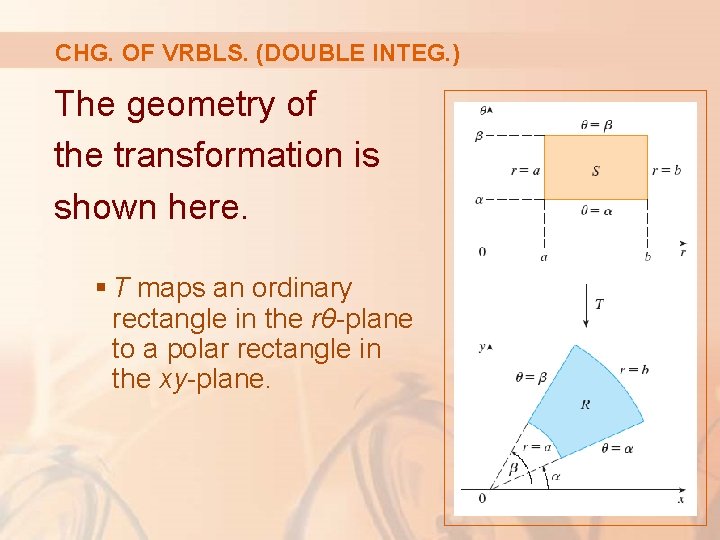
CHG. OF VRBLS. (DOUBLE INTEG. ) The geometry of the transformation is shown here. § T maps an ordinary rectangle in the rθ-plane to a polar rectangle in the xy-plane.

CHG. OF VRBLS. (DOUBLE INTEG. ) The Jacobian of T is:

CHG. OF VRBLS. (DOUBLE INTEG. ) So, Theorem 9 gives: § This is the same as Formula 2 in Section 15. 4

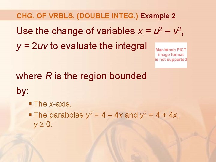
CHG. OF VRBLS. (DOUBLE INTEG. ) Example 2 Use the change of variables x = u 2 – v 2, y = 2 uv to evaluate the integral where R is the region bounded by: § The x-axis. § The parabolas y 2 = 4 – 4 x and y 2 = 4 + 4 x, y ≥ 0.

CHG. OF VRBLS. (DOUBLE INTEG. ) Example 2 The region R is pictured here.

CHG. OF VRBLS. (DOUBLE INTEG. ) Example 2 In Example 1, we discovered that T(S) = R where S is the square [0, 1] x [0, 1]. § Indeed, the reason for making the change of variables to evaluate the integral is that S is a much simpler region than R.

CHG. OF VRBLS. (DOUBLE INTEG. ) Example 2 First, we need to compute the Jacobian:

CHG. OF VRBLS. (DOUBLE INTEG. ) Example 2 So, by Theorem 9,

CHG. OF VRBLS. (DOUBLE INTEG. ) Note Example 2 was not very difficult to solve as we were given a suitable change of variables. If we are not supplied with a transformation, the first step is to think of an appropriate change of variables.

CHG. OF VRBLS. (DOUBLE INTEG. ) Note If f(x, y) is difficult to integrate, § The form of f(x, y) may suggest a transformation. If the region of integration R is awkward, § The transformation should be chosen so that the corresponding region S in the uv-plane has a convenient description.

CHG. OF VRBLS. (DOUBLE INTEG. ) Example 3 Evaluate the integral where R is the trapezoidal region with vertices (1, 0), (2, 0), (0, – 2), (0, – 1)

CHG. OF VRBLS. (DOUBLE INTEG. ) E. g. 3—Eqns. 10 It isn’t easy to integrate e(x+y)/(x–y). So, we make a change of variables suggested by the form of this function: u=x+y v=x–y § These equations define a transformation T– 1 from the xy-plane to the uv-plane.

CHG. OF VRBLS. (DOUBLE INTEG. ) E. g. 3—Equation 11 Theorem 9 talks about a transformation T from the uv-plane to the xy-plane. It is obtained by solving Equations 10 for x and y: x = ½(u + v) y = ½(u – v)

CHG. OF VRBLS. (DOUBLE INTEG. ) Example 3 The Jacobian of T is:

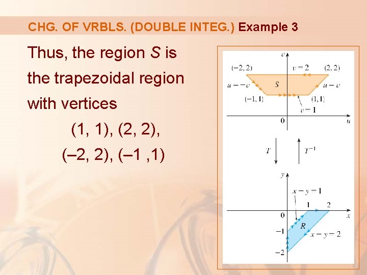
CHG. OF VRBLS. (DOUBLE INTEG. ) Example 3 To find the region S in the uv-plane corresponding to R, we note that: § The sides of R lie on the lines y=0 x–y=2 x=0 x–y=1 § From either Equations 10 or Equations 11, the image lines in the uv-plane are: u = v v = 2 u = –v v = 1

CHG. OF VRBLS. (DOUBLE INTEG. ) Example 3 Thus, the region S is the trapezoidal region with vertices (1, 1), (2, 2), (– 1 , 1)

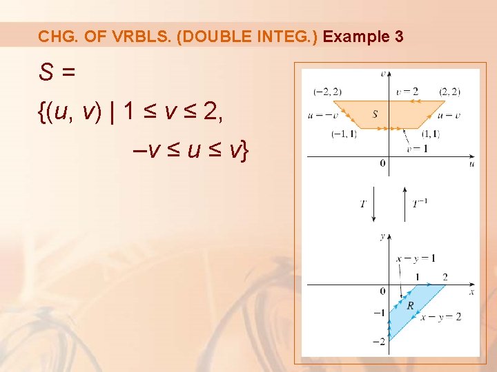
CHG. OF VRBLS. (DOUBLE INTEG. ) Example 3 S= {(u, v) | 1 ≤ v ≤ 2, –v ≤ u ≤ v}

CHG. OF VRBLS. (DOUBLE INTEG. ) Example 3 So, Theorem 9 gives:

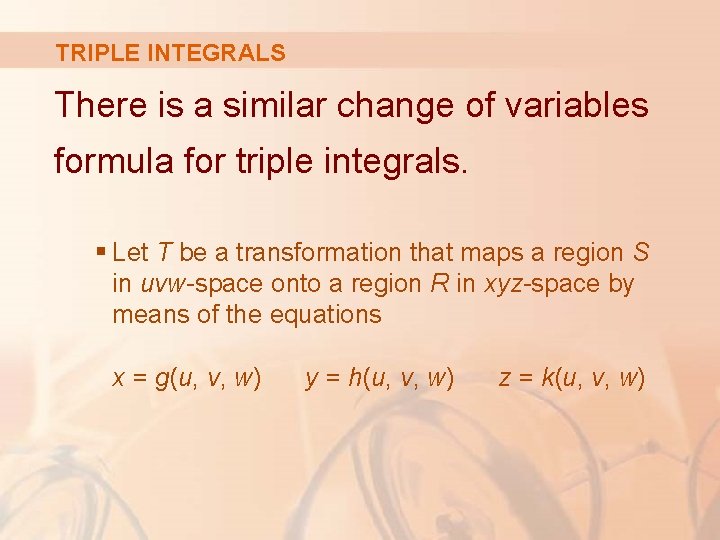
TRIPLE INTEGRALS There is a similar change of variables formula for triple integrals. § Let T be a transformation that maps a region S in uvw-space onto a region R in xyz-space by means of the equations x = g(u, v, w) y = h(u, v, w) z = k(u, v, w)

TRIPLE INTEGRALS Equation 12 The Jacobian of T is this 3 x 3 determinant:

TRIPLE INTEGRALS Formula 13 Under hypotheses similar to those in Theorem 9, we have this formula for triple integrals:

TRIPLE INTEGRALS Example 4 Use Formula 13 to derive the formula for triple integration in spherical coordinates. § The change of variables is given by: x = ρ sin Φ cos θ y = ρ sin Φ sin θ z = ρ cos Φ

TRIPLE INTEGRALS Example 4 We compute the Jacobian as follows:

TRIPLE INTEGRALS Example 4

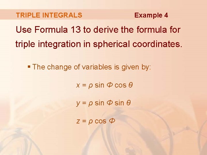
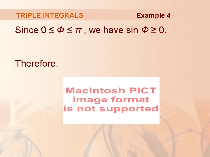
TRIPLE INTEGRALS Example 4 Since 0 ≤ Φ ≤ π , we have sin Φ ≥ 0. Therefore,

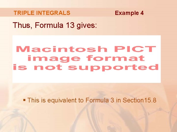
TRIPLE INTEGRALS Example 4 Thus, Formula 13 gives: § This is equivalent to Formula 3 in Section 15. 8