15 MULTIPLE INTEGRALS MULTIPLE INTEGRALS 15 5 Applications

15 MULTIPLE INTEGRALS

MULTIPLE INTEGRALS 15. 5 Applications of Double Integrals In this section, we will learn about: The physical applications of double integrals.

APPLICATIONS OF DOUBLE INTEGRALS We have already seen one application of double integrals: computing volumes. Another geometric application is finding areas of surfaces. § This will be done in Section 16. 6

APPLICATIONS OF DOUBLE INTEGRALS In this section, we explore physical applications—such as computing: § Mass § Electric charge § Center of mass § Moment of inertia

APPLICATIONS OF DOUBLE INTEGRALS We will see that these physical ideas are also important when applied to probability density functions of two random variables.

DENSITY AND MASS In Section 8. 3, we used single integrals to compute moments and the center of mass of a thin plate or lamina with constant density. Now, equipped with the double integral, we can consider a lamina with variable density.

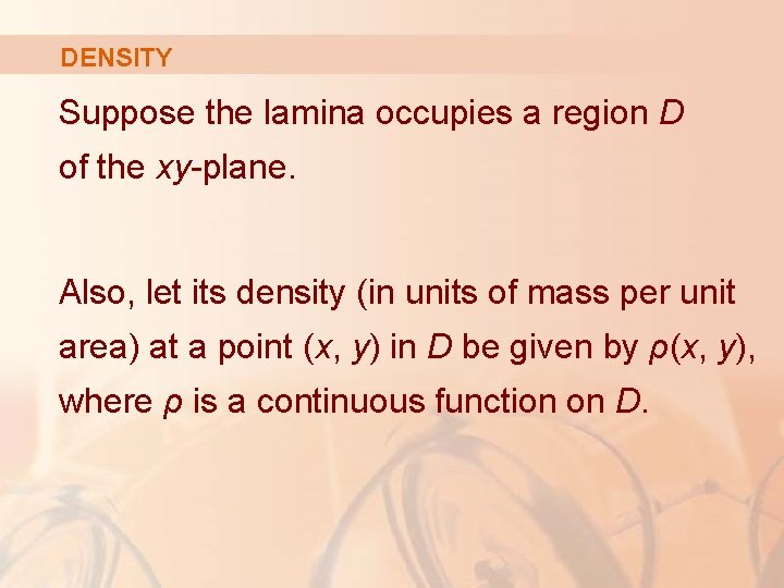
DENSITY Suppose the lamina occupies a region D of the xy-plane. Also, let its density (in units of mass per unit area) at a point (x, y) in D be given by ρ(x, y), where ρ is a continuous function on D.

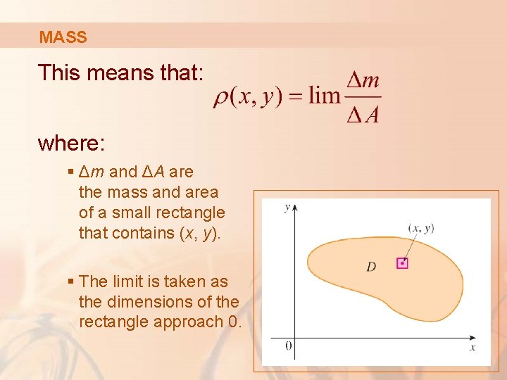
MASS This means that: where: § Δm and ΔA are the mass and area of a small rectangle that contains (x, y). § The limit is taken as the dimensions of the rectangle approach 0.

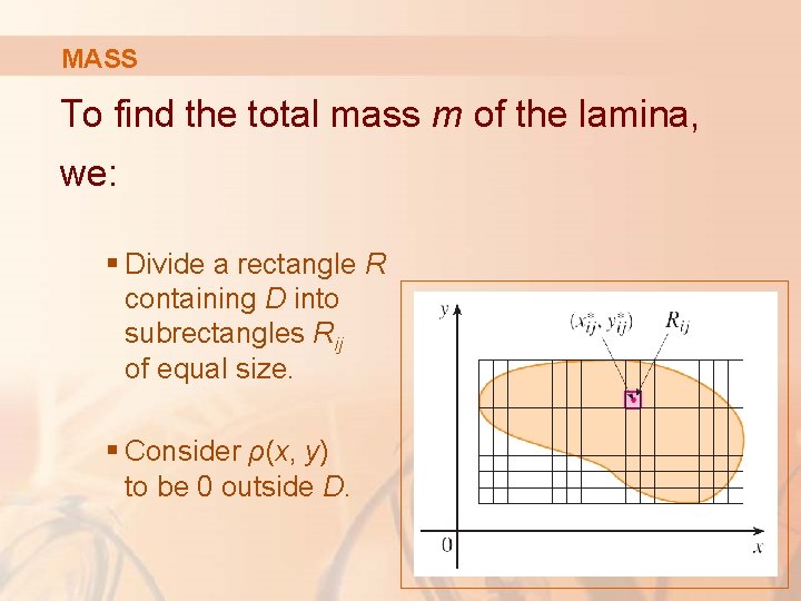
MASS To find the total mass m of the lamina, we: § Divide a rectangle R containing D into subrectangles Rij of equal size. § Consider ρ(x, y) to be 0 outside D.

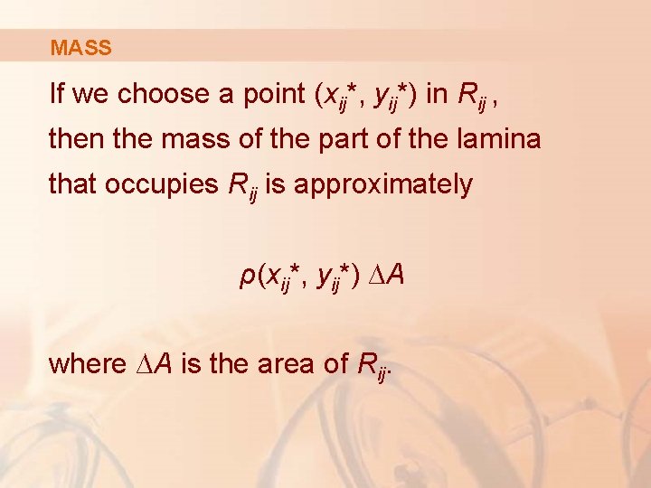
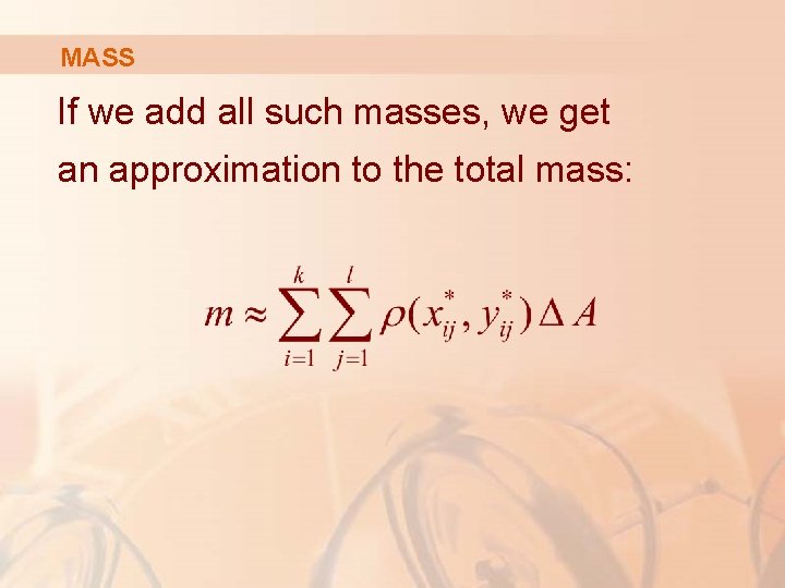
MASS If we choose a point (xij*, yij*) in Rij , then the mass of the part of the lamina that occupies Rij is approximately ρ(xij*, yij*) ∆A where ∆A is the area of Rij.

MASS If we add all such masses, we get an approximation to the total mass:

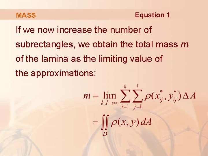
MASS Equation 1 If we now increase the number of subrectangles, we obtain the total mass m of the lamina as the limiting value of the approximations:

DENSITY AND MASS Physicists also consider other types of density that can be treated in the same manner. § For example, an electric charge is distributed over a region D and the charge density (in units of charge per unit area) is given by σ(x, y) at a point (x, y) in D.

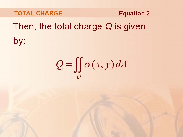
TOTAL CHARGE Equation 2 Then, the total charge Q is given by:

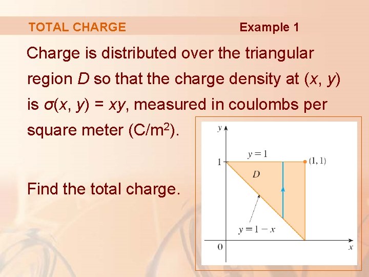
TOTAL CHARGE Example 1 Charge is distributed over the triangular region D so that the charge density at (x, y) is σ(x, y) = xy, measured in coulombs per square meter (C/m 2). Find the total charge.

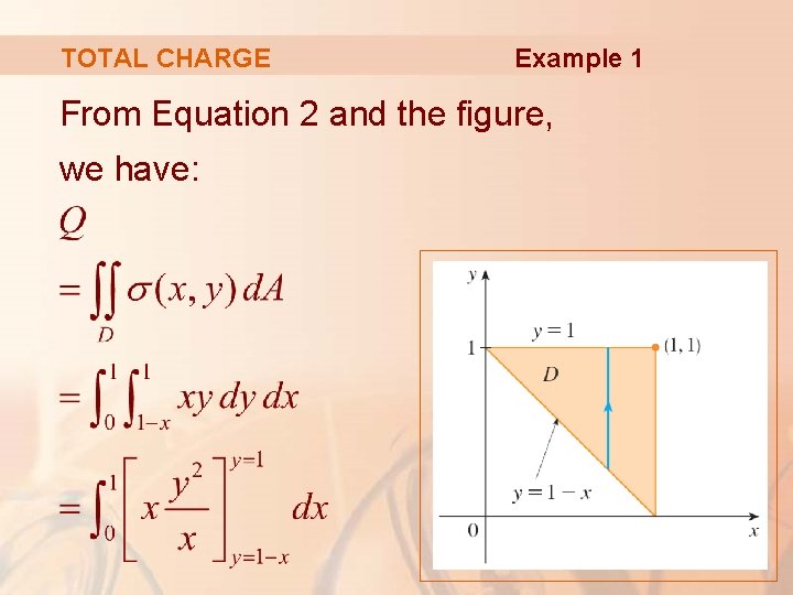
TOTAL CHARGE Example 1 From Equation 2 and the figure, we have:

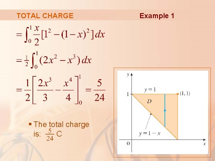
TOTAL CHARGE § The total charge is: C Example 1

MOMENTS AND CENTERS OF MASS In Section 8. 3, we found the center of mass of a lamina with constant density. Here, we consider a lamina with variable density.

MOMENTS AND CENTERS OF MASS Suppose the lamina occupies a region D and has density function ρ(x, y). § Recall from Chapter 8 that we defined the moment of a particle about an axis as the product of its mass and its directed distance from the axis.

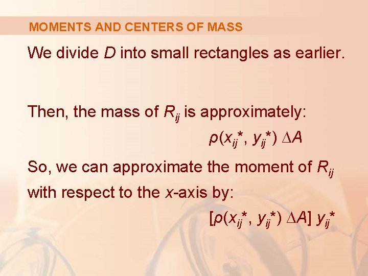
MOMENTS AND CENTERS OF MASS We divide D into small rectangles as earlier. Then, the mass of Rij is approximately: ρ(xij*, yij*) ∆A So, we can approximate the moment of Rij with respect to the x-axis by: [ρ(xij*, yij*) ∆A] yij*

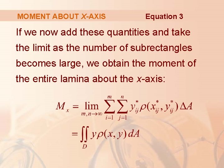
MOMENT ABOUT X-AXIS Equation 3 If we now add these quantities and take the limit as the number of subrectangles becomes large, we obtain the moment of the entire lamina about the x-axis:

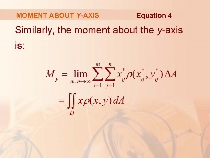
MOMENT ABOUT Y-AXIS Equation 4 Similarly, the moment about the y-axis is:

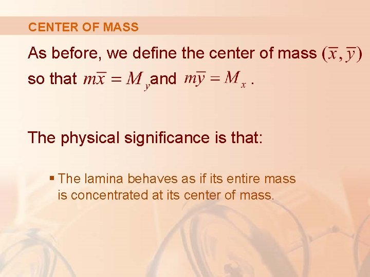
CENTER OF MASS As before, we define the center of mass so that and . The physical significance is that: § The lamina behaves as if its entire mass is concentrated at its center of mass.

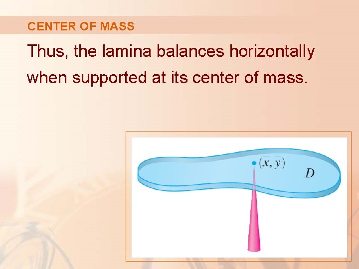
CENTER OF MASS Thus, the lamina balances horizontally when supported at its center of mass.

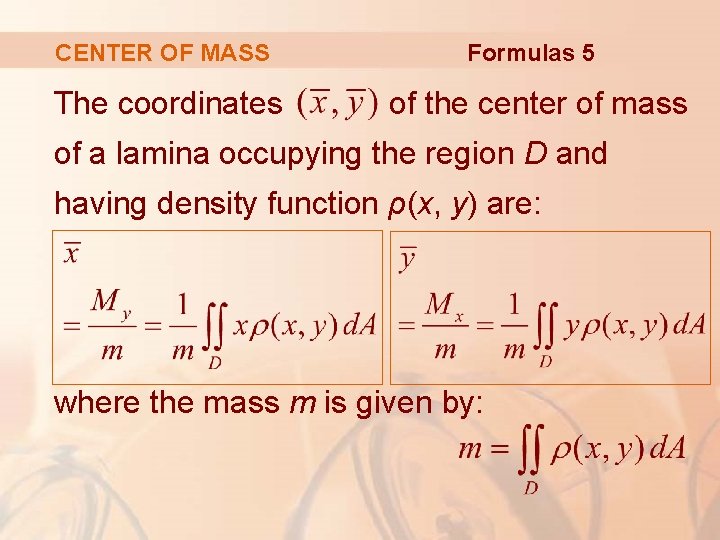
CENTER OF MASS The coordinates Formulas 5 of the center of mass of a lamina occupying the region D and having density function ρ(x, y) are: where the mass m is given by:

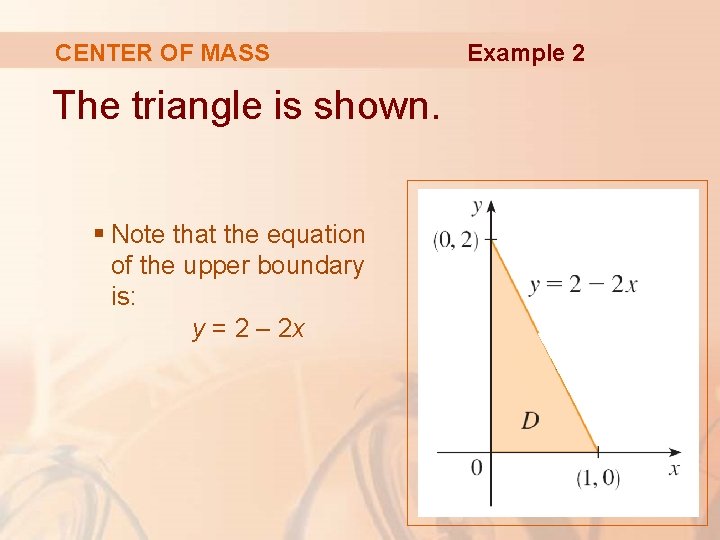
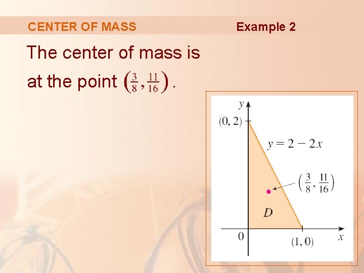
Example 2 CENTER OF MASS Find the mass and center of mass of a triangular lamina with vertices (0, 0), (1, 0), (0, 2) and if the density function is ρ(x, y) = 1 + 3 x + y

CENTER OF MASS The triangle is shown. § Note that the equation of the upper boundary is: y = 2 – 2 x Example 2

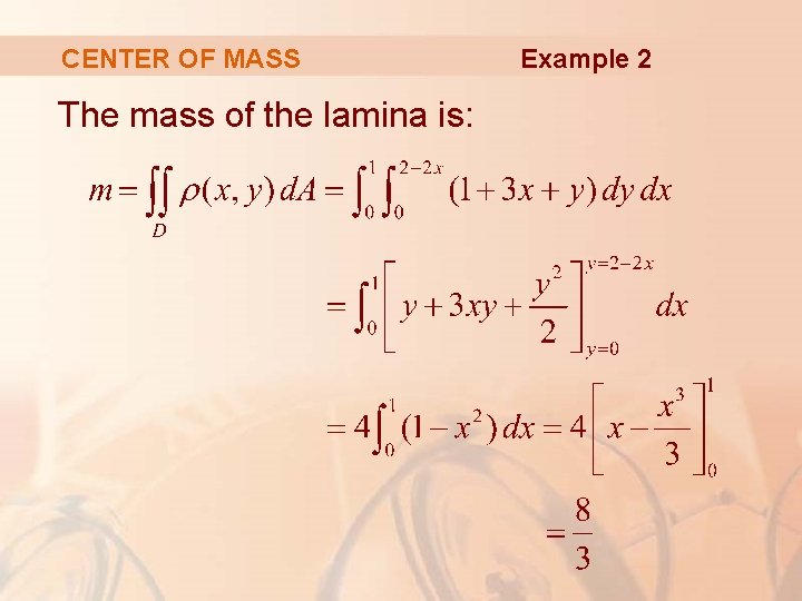
CENTER OF MASS The mass of the lamina is: Example 2

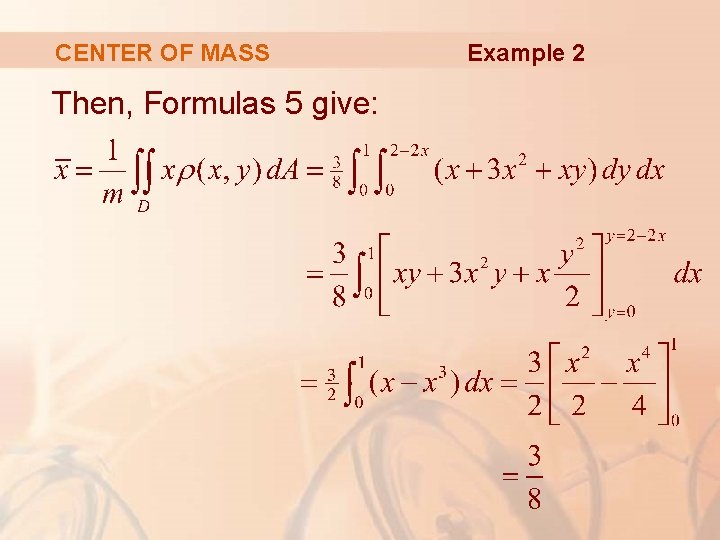
CENTER OF MASS Then, Formulas 5 give: Example 2

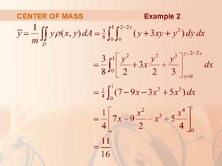
CENTER OF MASS Example 2

Example 2 CENTER OF MASS The center of mass is at the point .

CENTER OF MASS Example 3 The density at any point on a semicircular lamina is proportional to the distance from the center of the circle. Find the center of mass of the lamina.

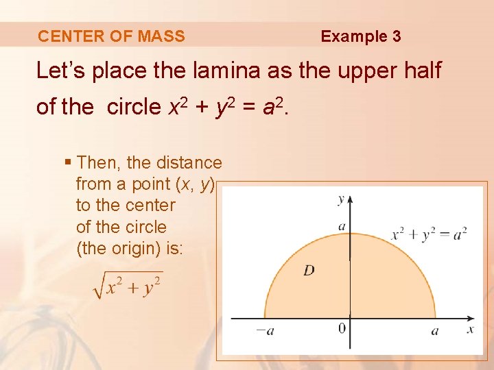
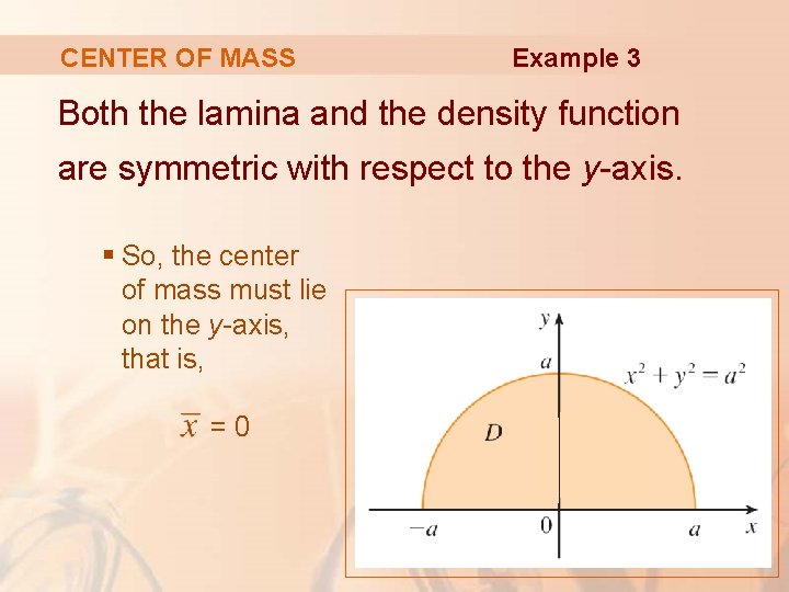
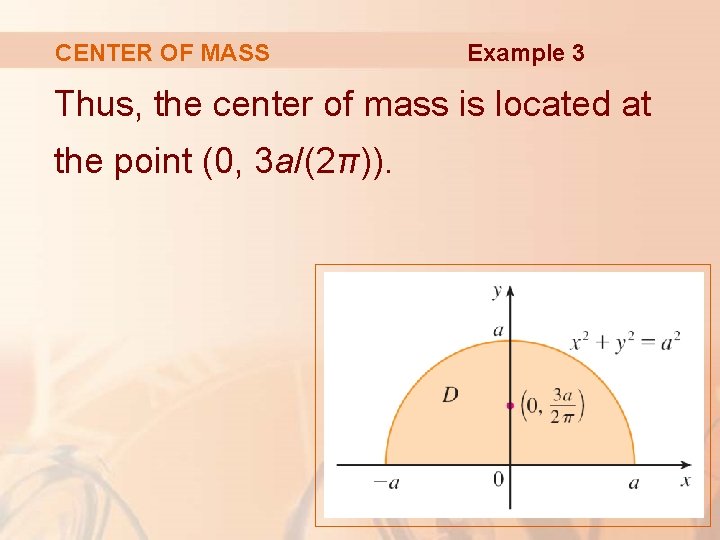
CENTER OF MASS Example 3 Let’s place the lamina as the upper half of the circle x 2 + y 2 = a 2. § Then, the distance from a point (x, y) to the center of the circle (the origin) is:

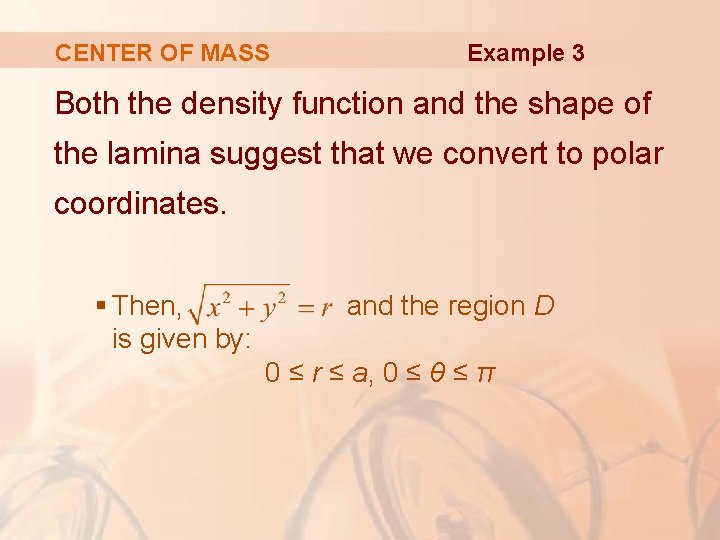
CENTER OF MASS Example 3 Therefore, the density function is: where K is some constant.

CENTER OF MASS Example 3 Both the density function and the shape of the lamina suggest that we convert to polar coordinates. § Then, is given by: and the region D 0 ≤ r ≤ a, 0 ≤ θ ≤ π

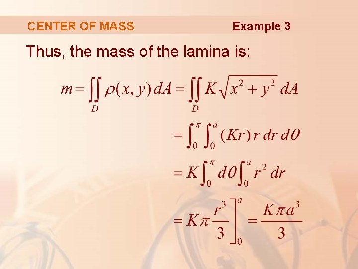
CENTER OF MASS Example 3 Thus, the mass of the lamina is:

CENTER OF MASS Example 3 Both the lamina and the density function are symmetric with respect to the y-axis. § So, the center of mass must lie on the y-axis, that is, =0

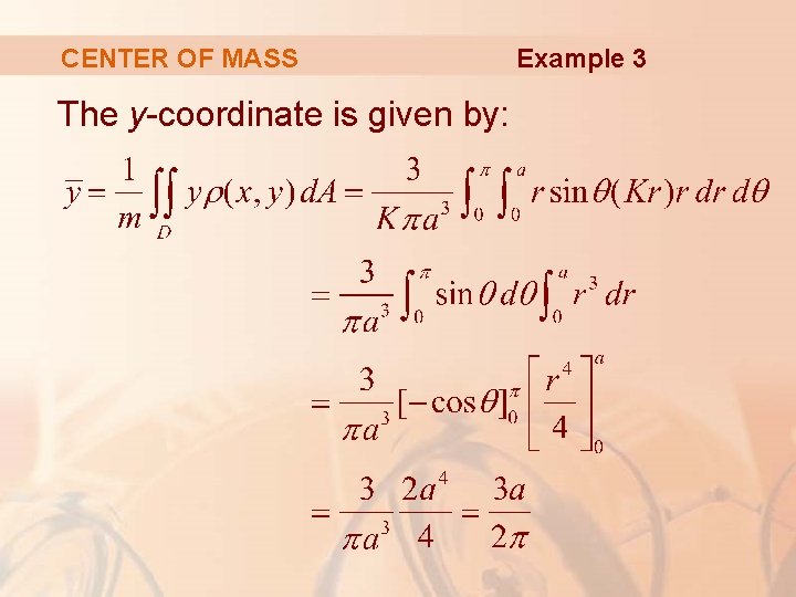
CENTER OF MASS The y-coordinate is given by: Example 3

CENTER OF MASS Example 3 Thus, the center of mass is located at the point (0, 3 a/(2π)).

MOMENT OF INERTIA The moment of inertia (also called the second moment) of a particle of mass m about an axis is defined to be mr 2, where r is the distance from the particle to the axis. § We extend this concept to a lamina with density function ρ(x, y) and occupying a region D by proceeding as we did for ordinary moments.

MOMENT OF INERTIA Thus, we: § Divide D into small rectangles. § Approximate the moment of inertia of each subrectangle about the x-axis. § Take the limit of the sum as the number of subrectangles becomes large.

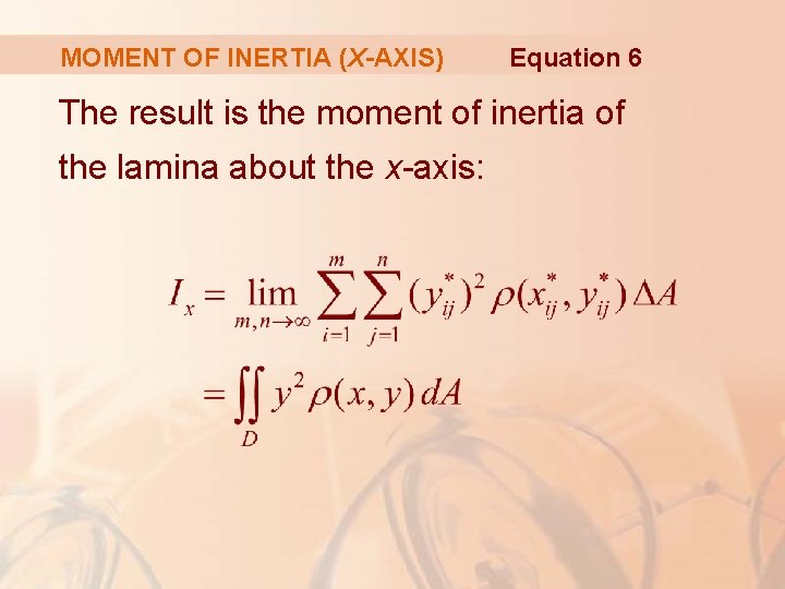
MOMENT OF INERTIA (X-AXIS) Equation 6 The result is the moment of inertia of the lamina about the x-axis:

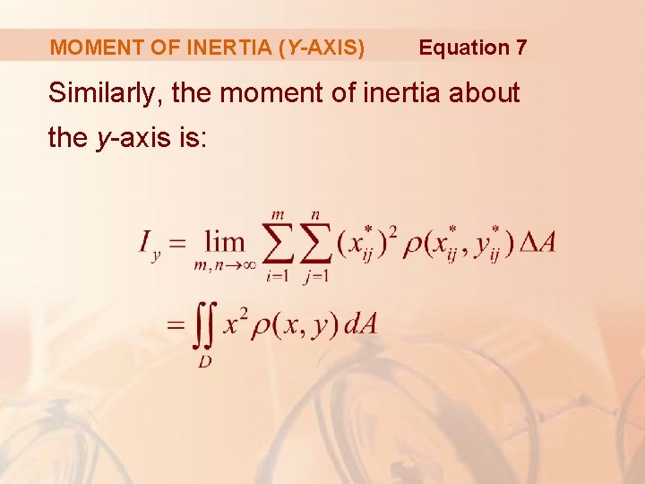
MOMENT OF INERTIA (Y-AXIS) Equation 7 Similarly, the moment of inertia about the y-axis is:

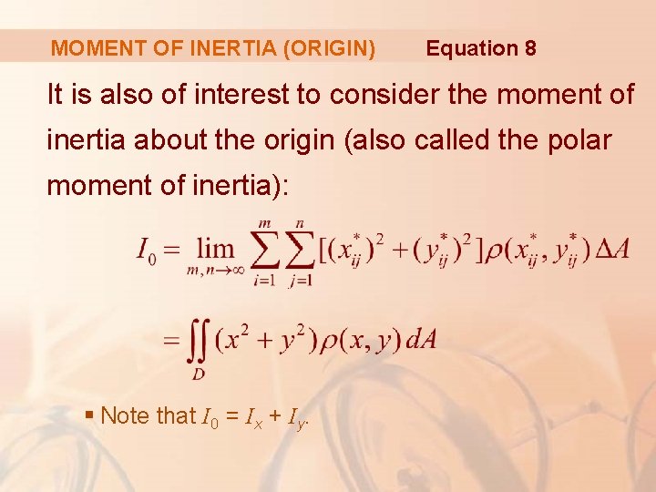
MOMENT OF INERTIA (ORIGIN) Equation 8 It is also of interest to consider the moment of inertia about the origin (also called the polar moment of inertia): § Note that I 0 = Ix + Iy.

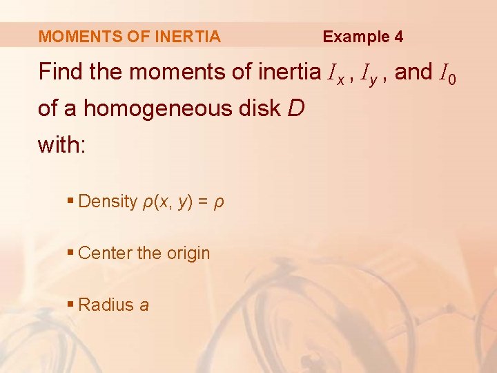
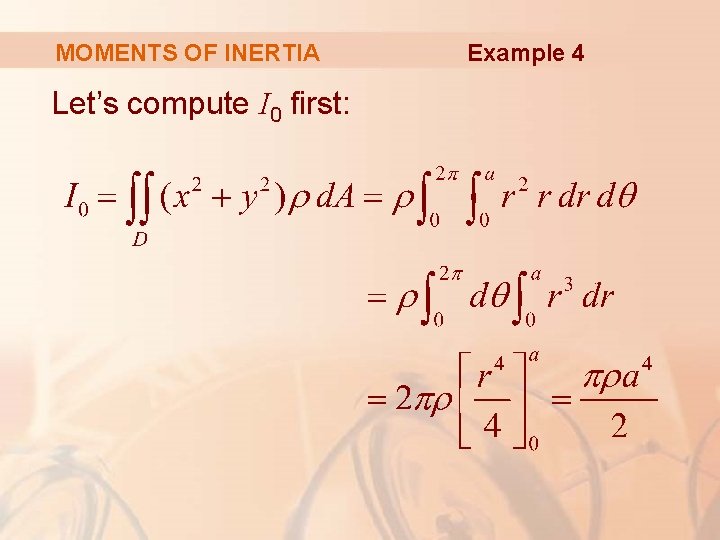
MOMENTS OF INERTIA Example 4 Find the moments of inertia Ix , Iy , and I 0 of a homogeneous disk D with: § Density ρ(x, y) = ρ § Center the origin § Radius a

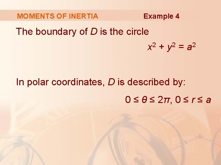
MOMENTS OF INERTIA Example 4 The boundary of D is the circle x 2 + y 2 = a 2 In polar coordinates, D is described by: 0 ≤ θ ≤ 2π, 0 ≤ r ≤ a

MOMENTS OF INERTIA Let’s compute I 0 first: Example 4

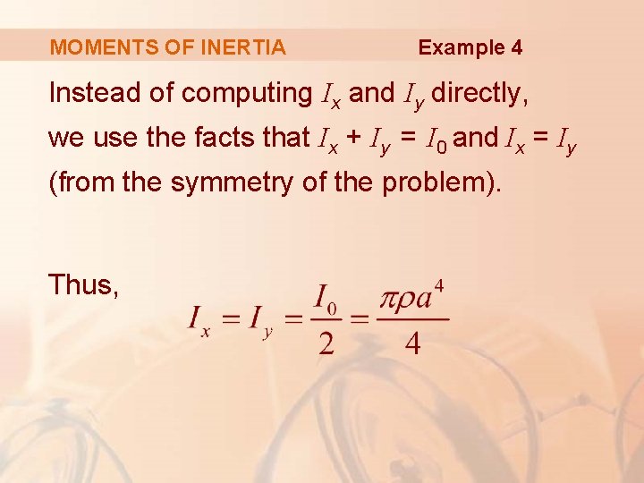
MOMENTS OF INERTIA Example 4 Instead of computing Ix and Iy directly, we use the facts that Ix + Iy = I 0 and Ix = Iy (from the symmetry of the problem). Thus,

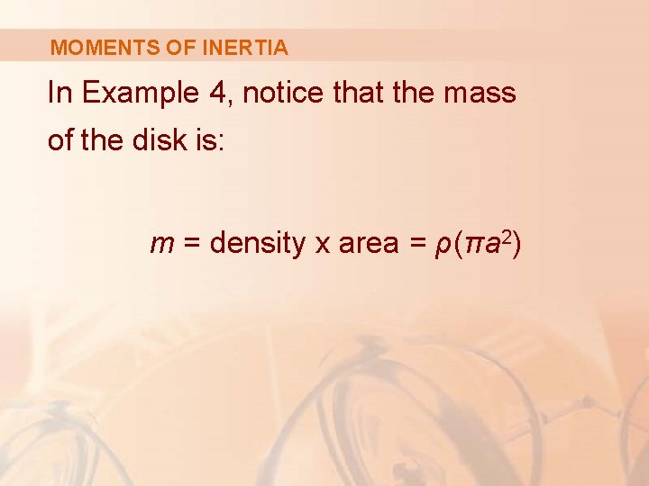
MOMENTS OF INERTIA In Example 4, notice that the mass of the disk is: m = density x area = ρ(πa 2)

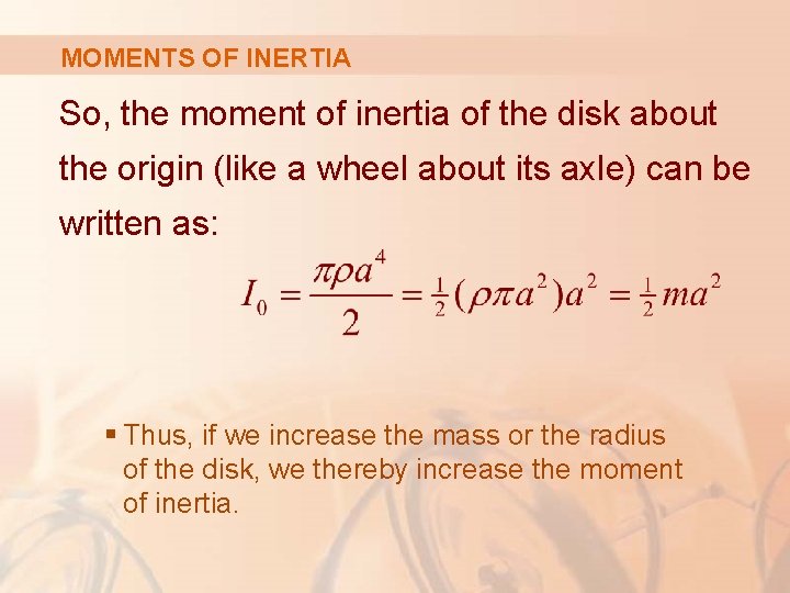
MOMENTS OF INERTIA So, the moment of inertia of the disk about the origin (like a wheel about its axle) can be written as: § Thus, if we increase the mass or the radius of the disk, we thereby increase the moment of inertia.

MOMENTS OF INERTIA In general, the moment of inertia plays much the same role in rotational motion that mass plays in linear motion. § The moment of inertia of a wheel is what makes it difficult to start or stop the rotation of the wheel. § This is just as the mass of a car is what makes it difficult to start or stop the motion of the car.

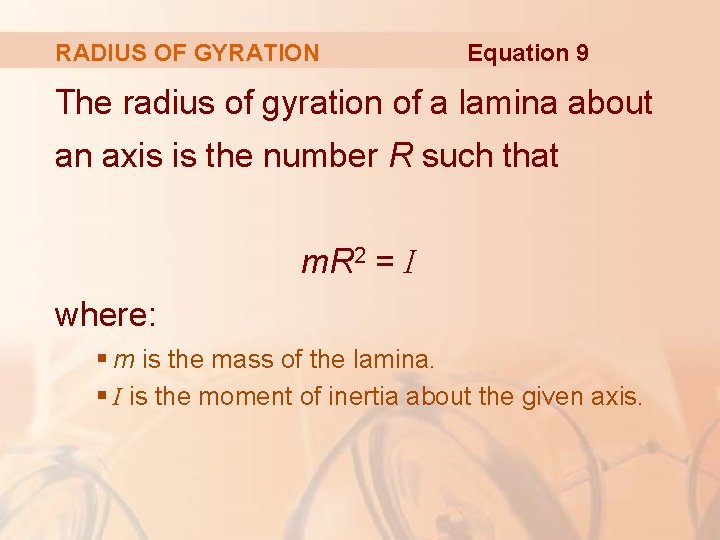
RADIUS OF GYRATION Equation 9 The radius of gyration of a lamina about an axis is the number R such that m. R 2 = I where: § m is the mass of the lamina. § I is the moment of inertia about the given axis.

RADIUS OF GYRATION Equation 9 says that: § If the mass of the lamina were concentrated at a distance R from the axis, then the moment of inertia of this “point mass” would be the same as the moment of inertia of the lamina.

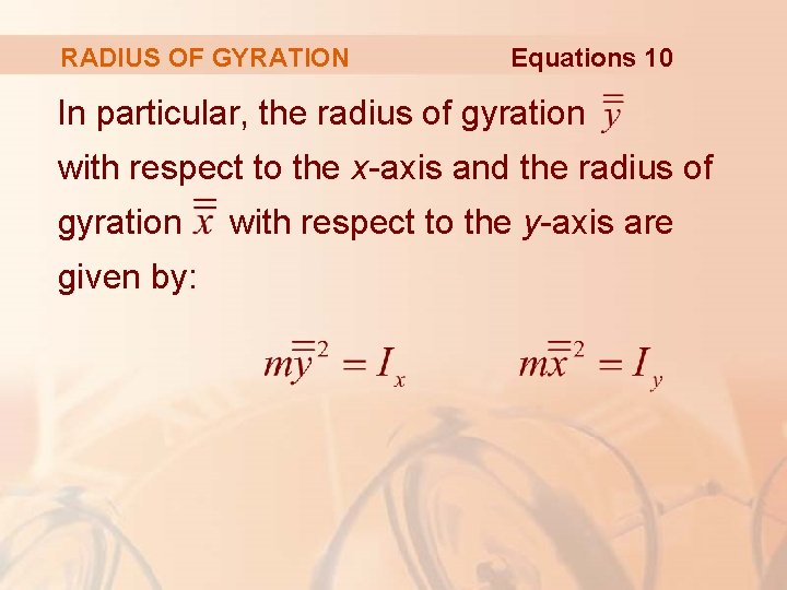
RADIUS OF GYRATION Equations 10 In particular, the radius of gyration with respect to the x-axis and the radius of gyration given by: with respect to the y-axis are

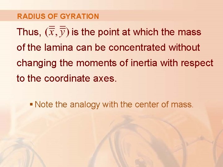
RADIUS OF GYRATION Thus, is the point at which the mass of the lamina can be concentrated without changing the moments of inertia with respect to the coordinate axes. § Note the analogy with the center of mass.

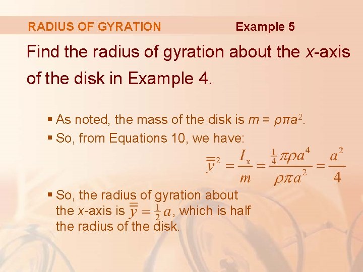
RADIUS OF GYRATION Example 5 Find the radius of gyration about the x-axis of the disk in Example 4. § As noted, the mass of the disk is m = ρπa 2. § So, from Equations 10, we have: § So, the radius of gyration about the x-axis is , which is half the radius of the disk.

PROBABILITY In Section 8. 5, we considered the probability density function f of a continuous random variable X.

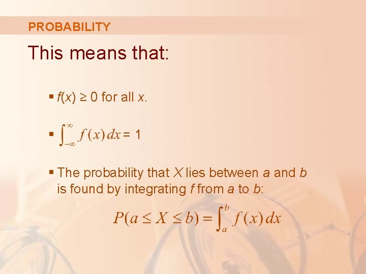
PROBABILITY This means that: § f(x) ≥ 0 for all x. § =1 § The probability that X lies between a and b is found by integrating f from a to b:

PROBABILITY Now, we consider a pair of continuous random variables X and Y, such as: § The lifetimes of two components of a machine. § The height and weight of an adult female chosen at random.

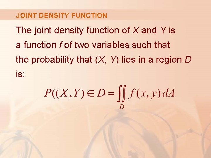
JOINT DENSITY FUNCTION The joint density function of X and Y is a function f of two variables such that the probability that (X, Y) lies in a region D is:

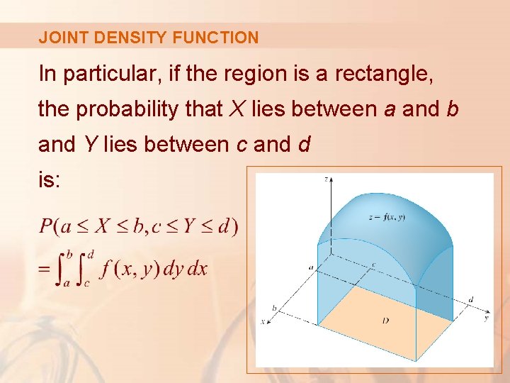
JOINT DENSITY FUNCTION In particular, if the region is a rectangle, the probability that X lies between a and b and Y lies between c and d is:

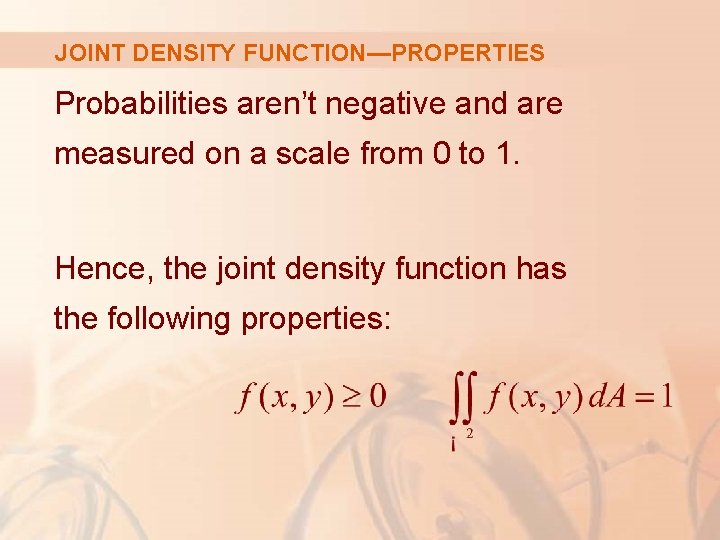
JOINT DENSITY FUNCTION—PROPERTIES Probabilities aren’t negative and are measured on a scale from 0 to 1. Hence, the joint density function has the following properties:

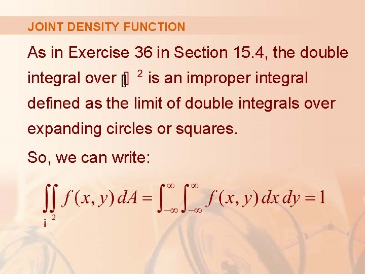
JOINT DENSITY FUNCTION As in Exercise 36 in Section 15. 4, the double integral over is an improper integral defined as the limit of double integrals over expanding circles or squares. So, we can write:

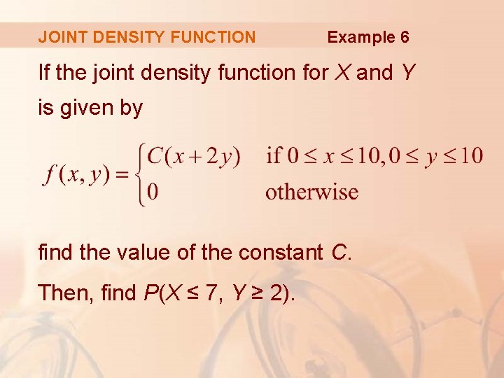
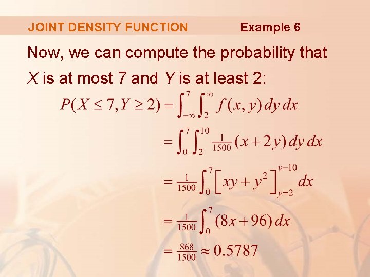
JOINT DENSITY FUNCTION Example 6 If the joint density function for X and Y is given by find the value of the constant C. Then, find P(X ≤ 7, Y ≥ 2).

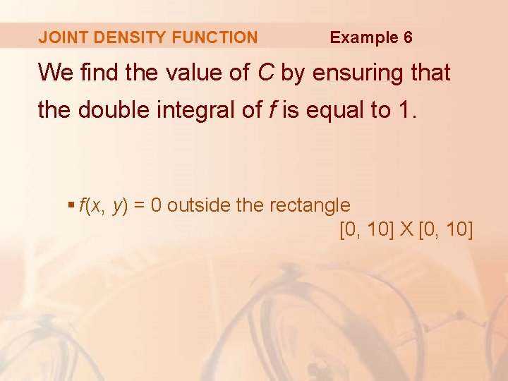
JOINT DENSITY FUNCTION Example 6 We find the value of C by ensuring that the double integral of f is equal to 1. § f(x, y) = 0 outside the rectangle [0, 10] X [0, 10]

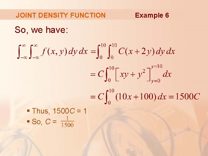
JOINT DENSITY FUNCTION So, we have: § Thus, 1500 C = 1 § So, C = Example 6

JOINT DENSITY FUNCTION Example 6 Now, we can compute the probability that X is at most 7 and Y is at least 2:

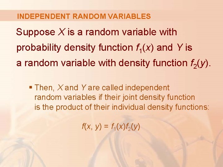
INDEPENDENT RANDOM VARIABLES Suppose X is a random variable with probability density function f 1(x) and Y is a random variable with density function f 2(y). § Then, X and Y are called independent random variables if their joint density function is the product of their individual density functions: f(x, y) = f 1(x)f 2(y)

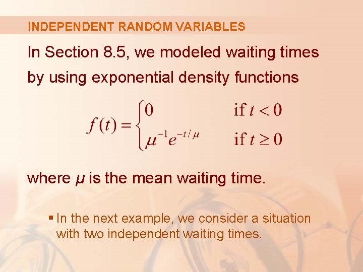
INDEPENDENT RANDOM VARIABLES In Section 8. 5, we modeled waiting times by using exponential density functions where μ is the mean waiting time. § In the next example, we consider a situation with two independent waiting times.

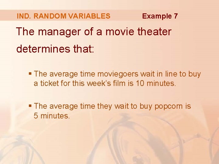
IND. RANDOM VARIABLES Example 7 The manager of a movie theater determines that: § The average time moviegoers wait in line to buy a ticket for this week’s film is 10 minutes. § The average time they wait to buy popcorn is 5 minutes.

IND. RANDOM VARIABLES Example 7 Assuming that the waiting times are independent, find the probability that a moviegoer waits a total of less than 20 minutes before taking his or her seat.

IND. RANDOM VARIABLES Example 7 Let’s assume that both the waiting time X for the ticket purchase and the waiting time Y in the refreshment line are modeled by exponential probability density functions.

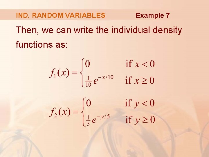
IND. RANDOM VARIABLES Example 7 Then, we can write the individual density functions as:

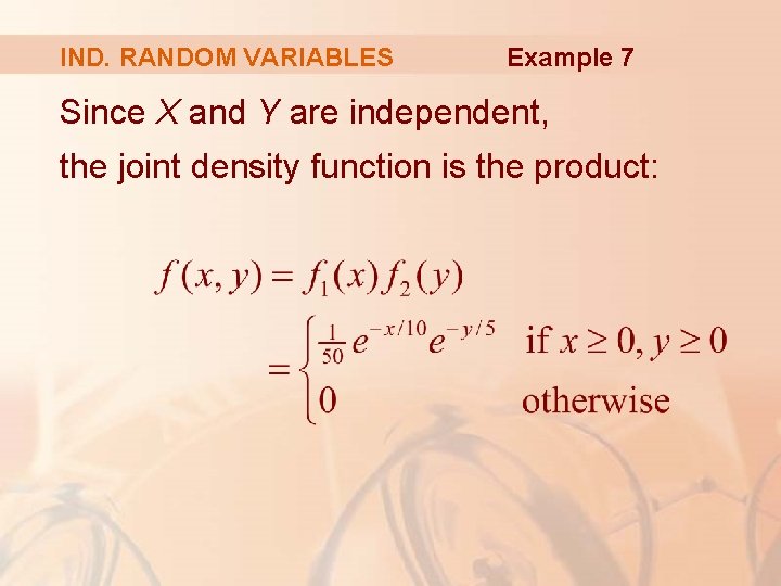
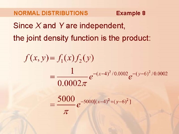
IND. RANDOM VARIABLES Example 7 Since X and Y are independent, the joint density function is the product:

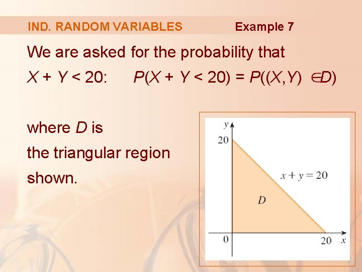
IND. RANDOM VARIABLES Example 7 We are asked for the probability that X + Y < 20: P(X + Y < 20) = P((X, Y) where D is the triangular region shown. D)

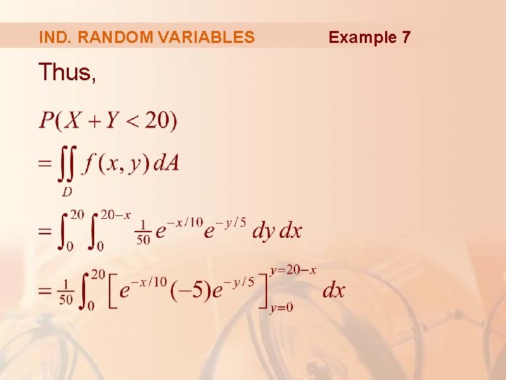
IND. RANDOM VARIABLES Thus, Example 7

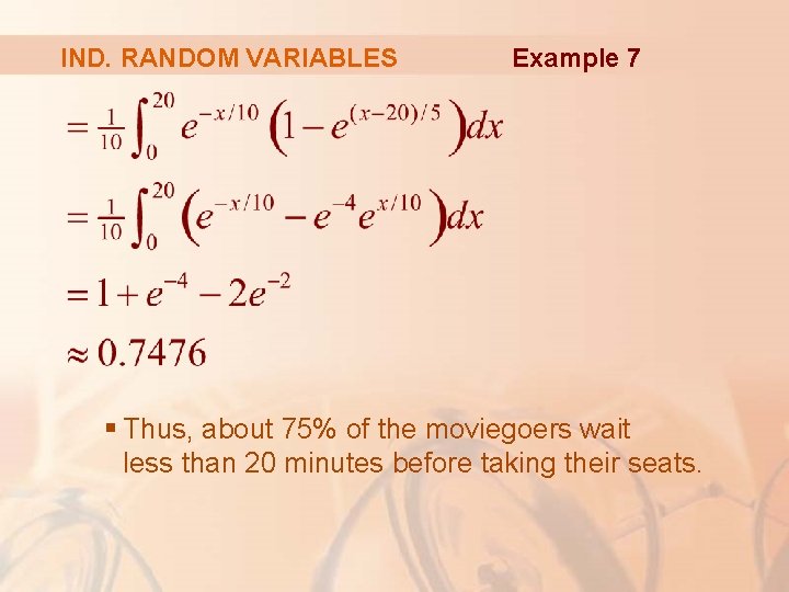
IND. RANDOM VARIABLES Example 7 § Thus, about 75% of the moviegoers wait less than 20 minutes before taking their seats.

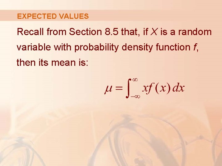
EXPECTED VALUES Recall from Section 8. 5 that, if X is a random variable with probability density function f, then its mean is:

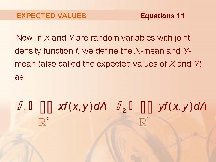
EXPECTED VALUES Equations 11 Now, if X and Y are random variables with joint density function f, we define the X-mean and Ymean (also called the expected values of X and Y) as:

EXPECTED VALUES Notice how closely the expressions for μ 1 and μ 2 in Equations 11 resemble the moments Mx and My of a lamina with density function ρ in Equations 3 and 4.

EXPECTED VALUES In fact, we can think of probability as being like continuously distributed mass. We calculate probability the way we calculate mass—by integrating a density function.

EXPECTED VALUES Then, as the total “probability mass” is 1, the expressions for and in Formulas 5 show that: § We can think of the expected values of X and Y, μ 1 and μ 2, as the coordinates of the “center of mass” of the probability distribution.

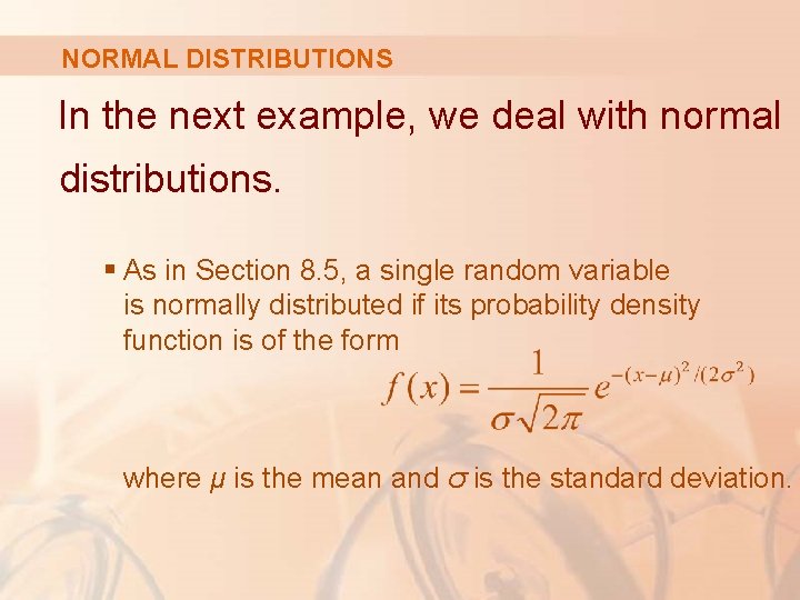
NORMAL DISTRIBUTIONS In the next example, we deal with normal distributions. § As in Section 8. 5, a single random variable is normally distributed if its probability density function is of the form where μ is the mean and σ is the standard deviation.

NORMAL DISTRIBUTIONS Example 8 A factory produces (cylindrically shaped) roller bearings that are sold as having diameter 4. 0 cm and length 6. 0 cm. § The diameters X are normally distributed with mean 4. 0 cm and standard deviation 0. 01 cm. § The lengths Y are normally distributed with mean 6. 0 cm and standard deviation 0. 01 cm.

NORMAL DISTRIBUTIONS Example 8 Assuming that X and Y are independent, write the joint density function and graph it. Find the probability that a bearing randomly chosen from the production line has either length or diameter that differs from the mean by more than 0. 02 cm.

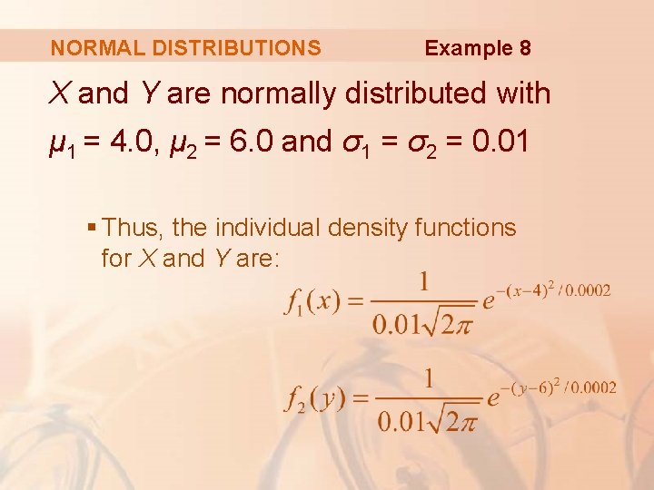
NORMAL DISTRIBUTIONS Example 8 X and Y are normally distributed with μ 1 = 4. 0, μ 2 = 6. 0 and σ1 = σ2 = 0. 01 § Thus, the individual density functions for X and Y are:

NORMAL DISTRIBUTIONS Example 8 Since X and Y are independent, the joint density function is the product:

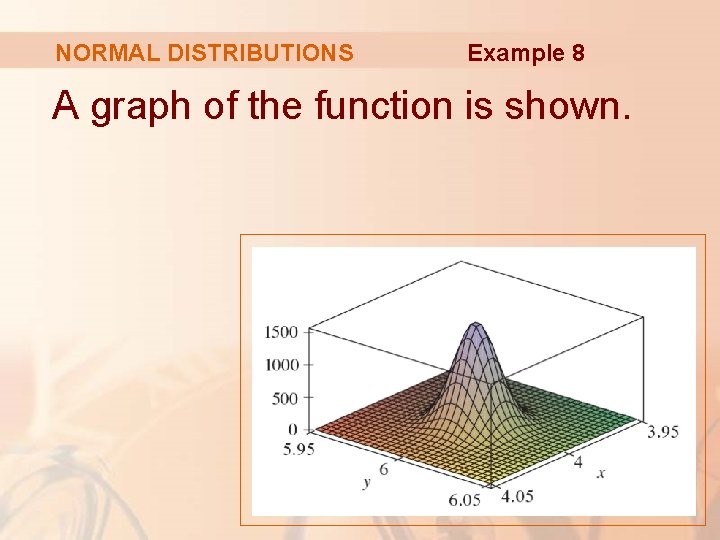
NORMAL DISTRIBUTIONS Example 8 A graph of the function is shown.

NORMAL DISTRIBUTIONS Example 8 Let’s first calculate the probability that both X and Y differ from their means by less than 0. 02 cm.

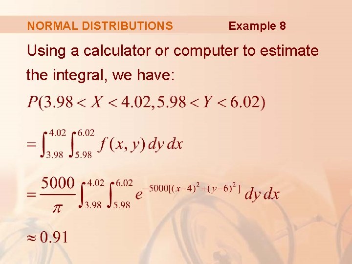
NORMAL DISTRIBUTIONS Example 8 Using a calculator or computer to estimate the integral, we have:

NORMAL DISTRIBUTIONS Example 8 Then, the probability that either X or Y differs from its mean by more than 0. 02 cm is approximately: 1 – 0. 91 = 0. 09