15 MathReview Friday 81800 1 Random Variables y

15. Math-Review Friday 8/18/00 1

Random Variables y. Event: x. In this setting we are talking about some uncertain event. The outcome of which is uncertain y. Outcome: x. The result of an observation of the event once the uncertainty has been resolved. y. Probability: x. The likelihood that certain outcome is realized for the event. y. Example: x. To roll a balanced 6 -sided die is an event. The number that appears on top of the die once its rolled it’s the outcome. And any outcome (any of the 6 sides) has a probability of 1/6. 15. Math-Review 2

Random Variables y. We have an uncertain event. y. If the outcome of the uncertainty is a number then it is called a random variable: y. Example: x. The result of the flip of a coin is uncertain event. We can obtain heads or tails. This is not a random variable. x. If we associate the variable X a value equal to 1 if the coin flip is head and 0 if the coin flip is tails, then X is a random variable. 15. Math-Review 3

Random Variables z A random process (or event) is one whose outcome cannot be specified in advance (except in probabilistic terms). z A random variable is a number that reflects the outcome of a random process. 15. Math-Review 4

Random Variables z A random variable can be discrete or continuous. y. Discrete: The values the random variable can take are fixed discrete amounts. Example: The number on top after the roll of a die can be 1, 2, 3, 4, 5 or 6. y. Continuous: The random variable can take any value in some interval. Example: If we draw a student at random in the class and record their height in principle we can obtain any number between. 5 meters and 2. 5 meters. (Very unlikely in the extremes) 15. Math-Review 5

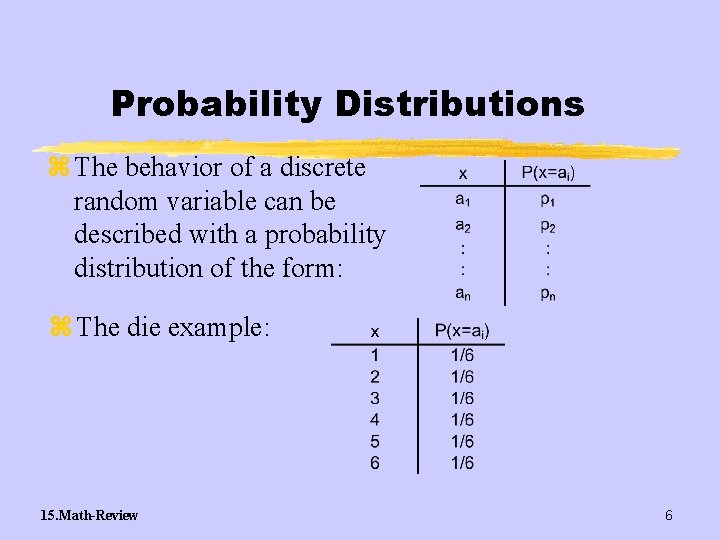
Probability Distributions z The behavior of a discrete random variable can be described with a probability distribution of the form: z The die example: 15. Math-Review 6

Probability Distributions z The probability that a continuous random variable takes exactly one value =0. y. There are infinite possible values the variable can take. z For a cont. r. v. we ask what is the probability that the r. v. falls within a certain interval. z If X is a cont. r. v. its cumulative distribution function F(x) is defined by: F(x) = P(X x) 15. Math-Review 7

Probability Distributions z What is P(a X b) for a cont. r. v. ? y. Since the events {X<a} and {a X b} are disjoint (mutually exclusive) we have: P(X b) = P({X<a} {a X b})=P(X<a)+P(a X b) = P(X a)+P(a X b) y. This means that P(a X b)= P(X b) - P(X a)=F(b)-F(a) 15. Math-Review 8

Probability Distributions z We define f (x) the probability density function of the cont. r. v. X as: z By construction we have that: z But what is this density function? 15. Math-Review 9

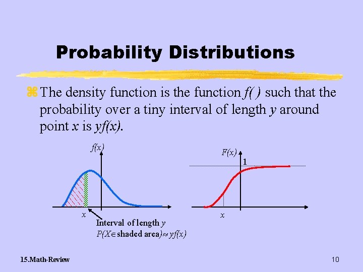
Probability Distributions z The density function is the function f( ) such that the probability over a tiny interval of length y around point x is yf(x) x 15. Math-Review Interval of length y P(X shaded area) yf(x) F(x) 1 x 10

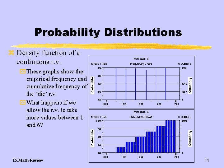
Probability Distributions z Density function of a continuous r. v. y These graphs show the empirical frequency and cumulative frequency of the ‘die’ r. v. y What happens if we allow the r. v. to take more values between 1 and 6? Forecast: 6 10, 000 Trials Frequency Chart 0 Outliers . 172 1715 . 129 . 086 857. 5 . 043 428. 7 . 000 0 0. 00 1. 75 3. 50 5. 25 7. 00 Forecast: 6 10, 000 Trials Cumulative Chart 0 Outliers 1. 000 10000 . 750 . 500 . 250 . 000 15. Math-Review 0 0. 00 1. 75 3. 50 5. 25 7. 00 11

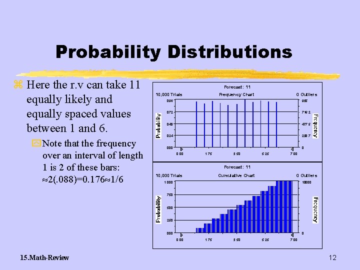
Probability Distributions z Here the r. v can take 11 equally likely and equally spaced values between 1 and 6. y Note that the frequency over an interval of length 1 is 2 of these bars: 2(. 088)=0. 176 1/6 Forecast: 11 10, 000 Trials Frequency Chart 0 Outliers . 096 955 . 072 716. 2 . 048 477. 5 . 024 238. 7 . 000 0 0. 00 1. 75 3. 50 5. 25 7. 00 Forecast: 11 10, 000 Trials Cumulative Chart 0 Outliers 1. 000 10000 . 750 . 500 . 250 . 000 0 0. 00 15. Math-Review 1. 75 3. 50 5. 25 7. 00 12

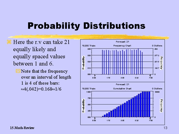
Probability Distributions z Here the r. v can take 21 equally likely and equally spaced values between 1 and 6. y Note that the frequency over an interval of length 1 is 4 of these bars: 4(. 042)=0. 168 1/6 Forecast: 21 10, 000 Trials Frequency Chart 0 Outliers . 050 503 . 038 377. 2 . 025 251. 5 . 013 125. 7 . 000 0 0. 00 1. 75 3. 50 5. 25 7. 00 Forecast: 21 10, 000 Trials Cumulative Chart 0 Outliers 1. 000 10000 . 750 . 500 . 250 . 000 0 0. 00 15. Math-Review 1. 75 3. 50 5. 25 7. 00 13

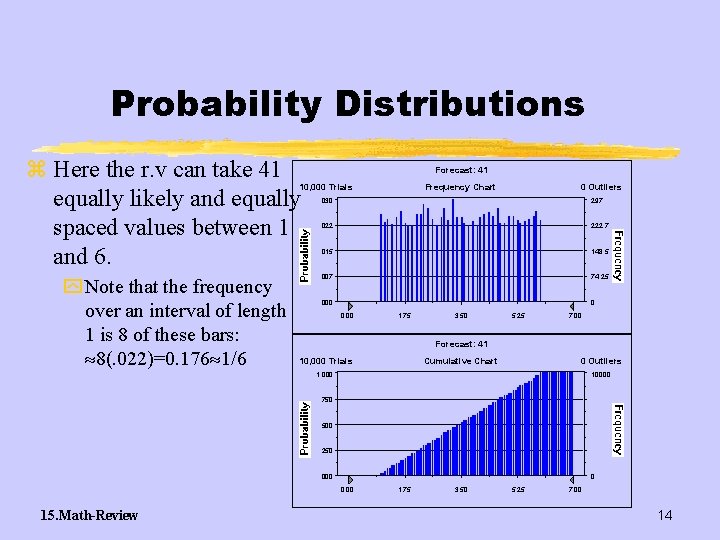
Probability Distributions z Here the r. v can take 41 equally likely and equally spaced values between 1 and 6. Forecast: 41 10, 000 Trials y Note that the frequency over an interval of length 1 is 8 of these bars: 8(. 022)=0. 176 1/6 Frequency Chart 0 Outliers . 030 297 . 022 222. 7 . 015 148. 5 . 007 74. 25 . 000 0 0. 00 1. 75 3. 50 5. 25 7. 00 Forecast: 41 10, 000 Trials Cumulative Chart 0 Outliers 1. 000 10000 . 750 . 500 . 250 . 000 0 0. 00 15. Math-Review 1. 75 3. 50 5. 25 7. 00 14

Probability Distributions z The probability of any one value decreases to 0. z The cumulative frequency function is smoother. z In the limit, when we pass to a continuous distribution: ythe cumulative frequency function will become the cumulative distribution function. y. The frequency function will go to the function g(x)=0. y. The frequency in an interval of length y will be y/6. 15. Math-Review 15

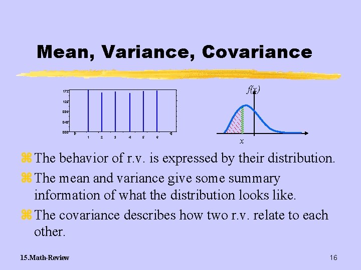
Mean, Variance, Covariance f(x) . 172. 129. 086. 043. 000 1 2 3 4 5 6 x z The behavior of r. v. is expressed by their distribution. z The mean and variance give some summary information of what the distribution looks like. z The covariance describes how two r. v. relate to each other. 15. Math-Review 16

Mean, Variance, Covariance z The mean of r. v. X is an average of the possible values of X weighted by the probability. y. In the discrete case: x. If X can take the values x 1, x 2, …, xn with probabilities p 1, p 2, …, pn respectively. y. In the continuous case: x. Where f(x) is the probability density function: 15. Math-Review 17

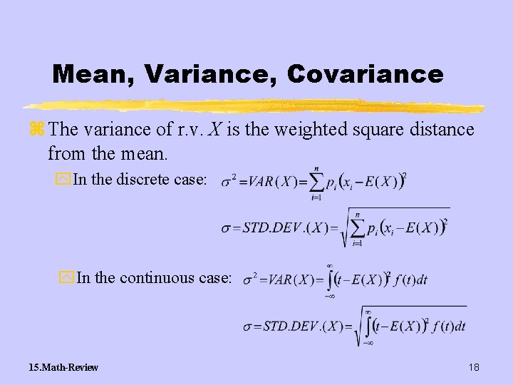
Mean, Variance, Covariance z The variance of r. v. X is the weighted square distance from the mean. y. In the discrete case: y. In the continuous case: 15. Math-Review 18

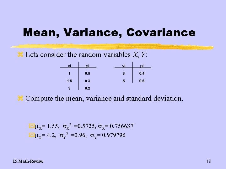
Mean, Variance, Covariance z Lets consider the random variables X, Y: z Compute the mean, variance and standard deviation. y X= 1. 55, X 2 =0. 5725, X= 0. 756637 y Y= 4. 2, Y 2 =0. 96, Y= 0. 979796 15. Math-Review 19

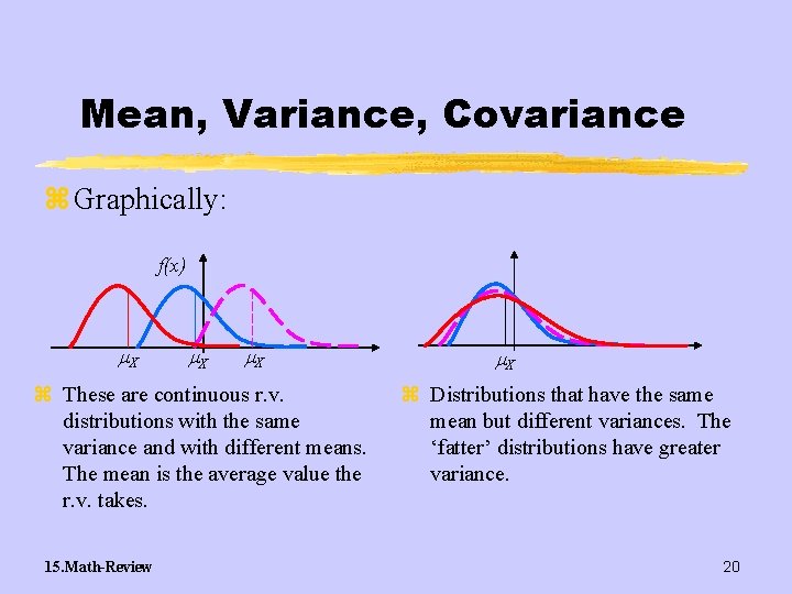
Mean, Variance, Covariance z Graphically: f(x) X X X z These are continuous r. v. distributions with the same variance and with different means. The mean is the average value the r. v. takes. 15. Math-Review X z Distributions that have the same mean but different variances. The ‘fatter’ distributions have greater variance. 20

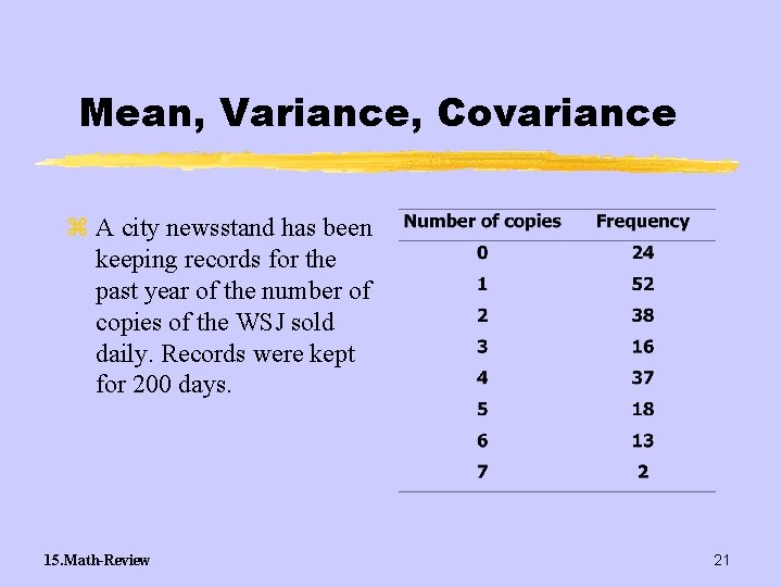
Mean, Variance, Covariance z A city newsstand has been keeping records for the past year of the number of copies of the WSJ sold daily. Records were kept for 200 days. 15. Math-Review 21

Mean, Variance, Covariance z What is the distribution of the number of copies of the WSJ sold in one day? z What is the average number of WSJ sold in one day? z What is the standard deviation of the number of WSJ sold each day? 15. Math-Review 22

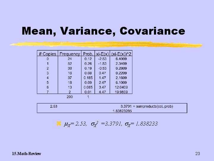
Mean, Variance, Covariance z X= 2. 53, X 2 =3. 3791, X= 1. 838233 15. Math-Review 23

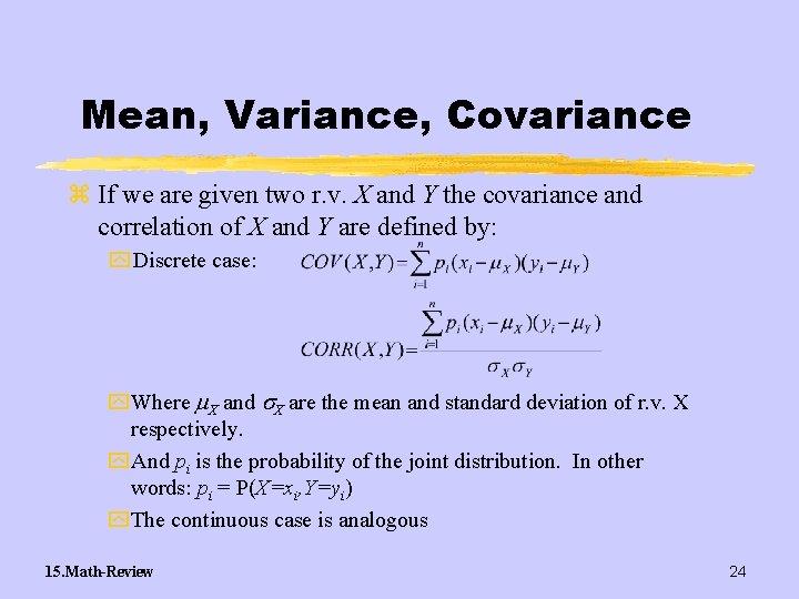
Mean, Variance, Covariance z If we are given two r. v. X and Y the covariance and correlation of X and Y are defined by: y Discrete case: y Where X and X are the mean and standard deviation of r. v. X respectively. y And pi is the probability of the joint distribution. In other words: pi = P(X=xi, Y=yi) y The continuous case is analogous 15. Math-Review 24

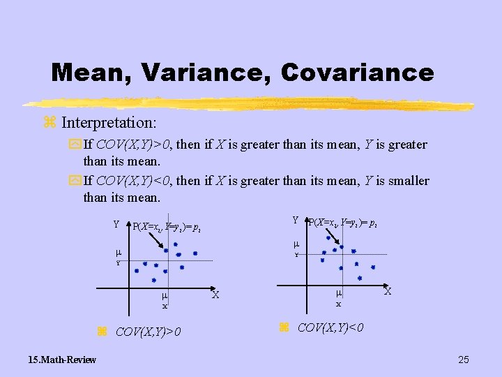
Mean, Variance, Covariance z Interpretation: y If COV(X, Y)>0, then if X is greater than its mean, Y is greater than its mean. y If COV(X, Y)<0, then if X is greater than its mean, Y is smaller than its mean. Y Y P(X=xi, , Y=yi )= pi Y Y X z COV(X, Y)>0 15. Math-Review X X X z COV(X, Y)<0 25

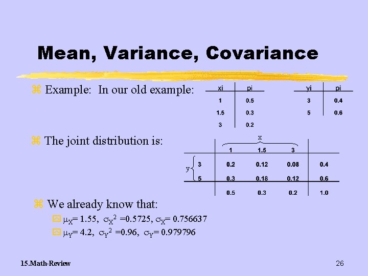
Mean, Variance, Covariance z Example: In our old example: x z The joint distribution is: y z We already know that: y X= 1. 55, X 2 =0. 5725, X= 0. 756637 y Y= 4. 2, Y 2 =0. 96, Y= 0. 979796 15. Math-Review 26

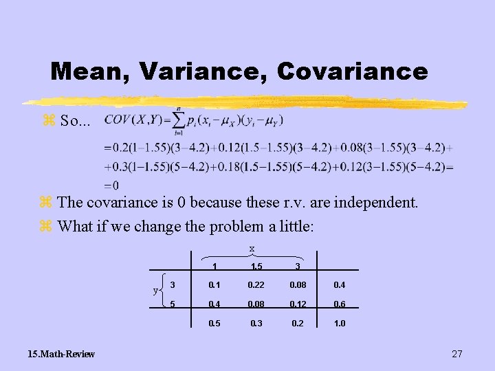
Mean, Variance, Covariance z So. . . z The covariance is 0 because these r. v. are independent. z What if we change the problem a little: x y 15. Math-Review 1 1. 5 3 3 0. 1 0. 22 0. 08 0. 4 5 0. 4 0. 08 0. 12 0. 6 0. 5 0. 3 0. 2 1. 0 27

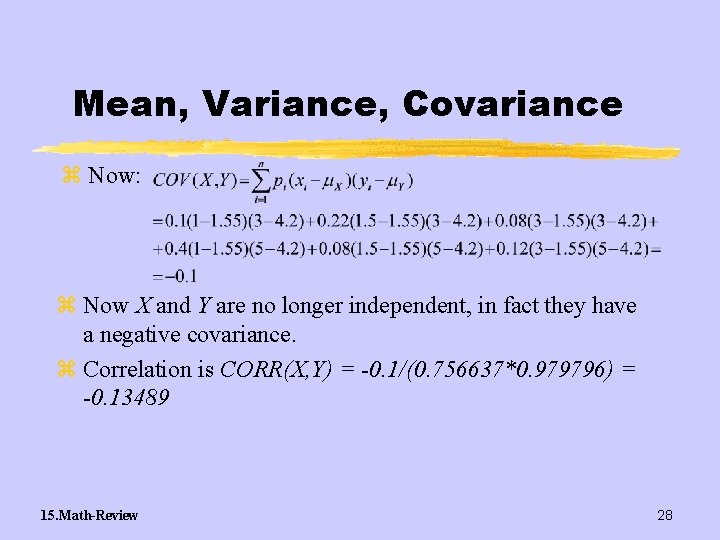
Mean, Variance, Covariance z Now: z Now X and Y are no longer independent, in fact they have a negative covariance. z Correlation is CORR(X, Y) = -0. 1/(0. 756637*0. 979796) = -0. 13489 15. Math-Review 28

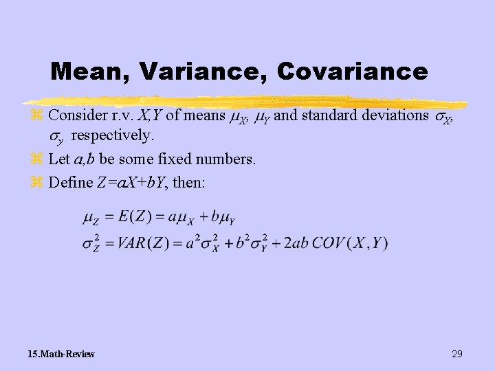
Mean, Variance, Covariance z Consider r. v. X, Y of means X, Y and standard deviations X, y respectively. z Let a, b be some fixed numbers. z Define Z=a. X+b. Y, then: 15. Math-Review 29

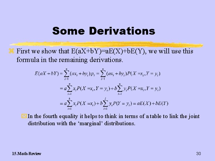
Some Derivations z First we show that E(a. X+b. Y)=a. E(X)+b. E(Y), we will use this formula in the remaining derivations. y In the fourth equality it helps to think in terms of a table to link the joint distribution with the ‘marginal’ distributions. 15. Math-Review 30

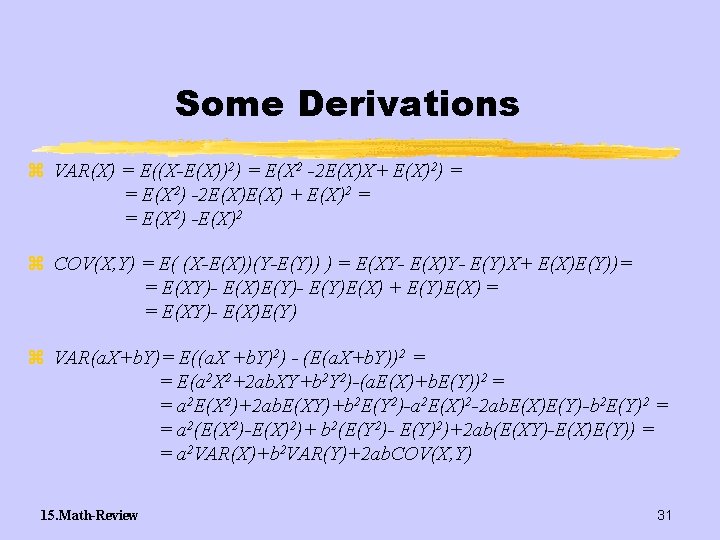
Some Derivations z VAR(X) = E((X-E(X))2) = E(X 2 -2 E(X)X+ E(X)2) = = E(X 2) -2 E(X) + E(X)2 = = E(X 2) -E(X)2 z COV(X, Y) = E( (X-E(X))(Y-E(Y)) ) = E(XY- E(X)Y- E(Y)X+ E(X)E(Y))= = E(XY)- E(X)E(Y)- E(Y)E(X) + E(Y)E(X) = = E(XY)- E(X)E(Y) z VAR(a. X+b. Y)= E((a. X +b. Y)2) - (E(a. X+b. Y))2 = = E(a 2 X 2+2 ab. XY+b 2 Y 2)-(a. E(X)+b. E(Y))2 = = a 2 E(X 2)+2 ab. E(XY)+b 2 E(Y 2)-a 2 E(X)2 -2 ab. E(X)E(Y)-b 2 E(Y)2 = = a 2(E(X 2)-E(X)2)+ b 2(E(Y 2)- E(Y)2)+2 ab(E(XY)-E(X)E(Y)) = = a 2 VAR(X)+b 2 VAR(Y)+2 ab. COV(X, Y) 15. Math-Review 31

Mean, Variance, Covariance z We know that an investment in Snowboard Inc. has a return that is a random variable with mean. 9 and standard deviation 0. 075. Also an investment in Skiboots Inc. has a return that is a random variable that we know has mean. 9 and standard deviation 0. 27. Also the return for these stocks has a correlation of -0. 75. z If you decide to invest 30% of your capital in Snowboard Inc, and 70% in Skiboots Inc. What is the mean and variance of the return of the resulting portfolio? z What if you invest 50% on each? 15. Math-Review 32