15 Linear Regression Expected change in Y per

15: Linear Regression Expected change in Y per unit X

Introduction (p. 15. 1) • X = independent (explanatory) variable • Y = dependent (response) variable • Use instead of correlation when distribution of X is fixed by researcher (i. e. , set number at each level of X) studying functional dependency between X and Y

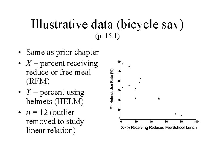
Illustrative data (bicycle. sav) (p. 15. 1) • Same as prior chapter • X = percent receiving reduce or free meal (RFM) • Y = percent using helmets (HELM) • n = 12 (outlier removed to study linear relation)

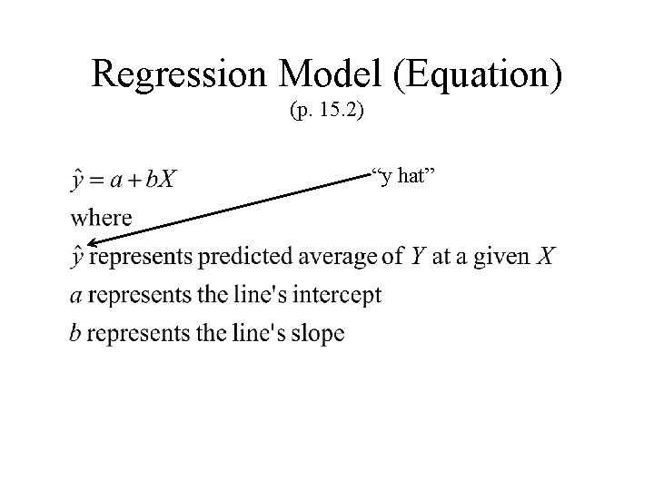
Regression Model (Equation) (p. 15. 2) “y hat”

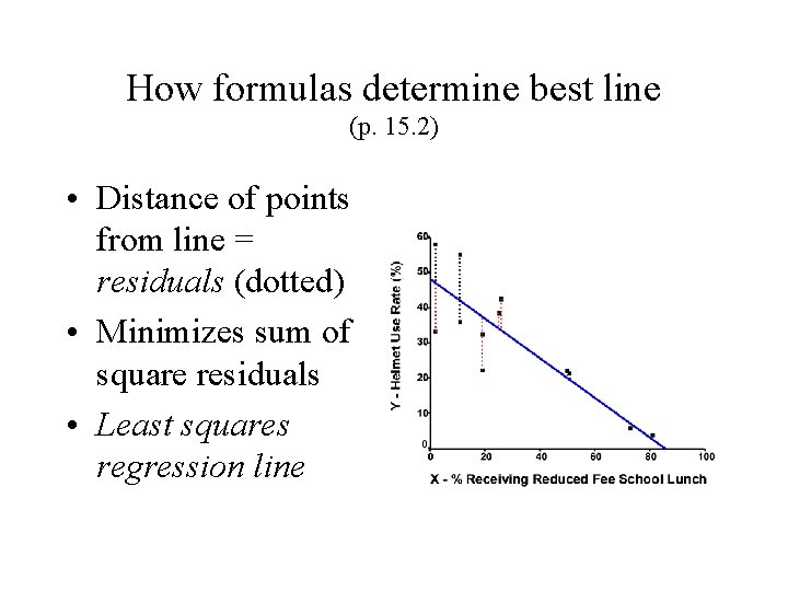
How formulas determine best line (p. 15. 2) • Distance of points from line = residuals (dotted) • Minimizes sum of square residuals • Least squares regression line

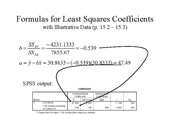
Formulas for Least Squares Coefficients with Illustrative Data (p. 15. 2 – 15. 3) SPSS output:

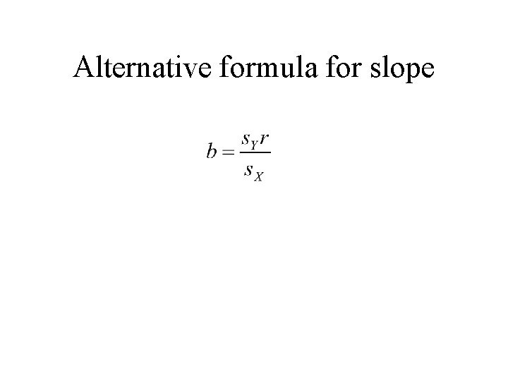
Alternative formula for slope

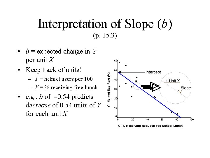
Interpretation of Slope (b) (p. 15. 3) • b = expected change in Y per unit X • Keep track of units! – Y = helmet users per 100 – X = % receiving free lunch • e. g. , b of – 0. 54 predicts decrease of 0. 54 units of Y for each unit X

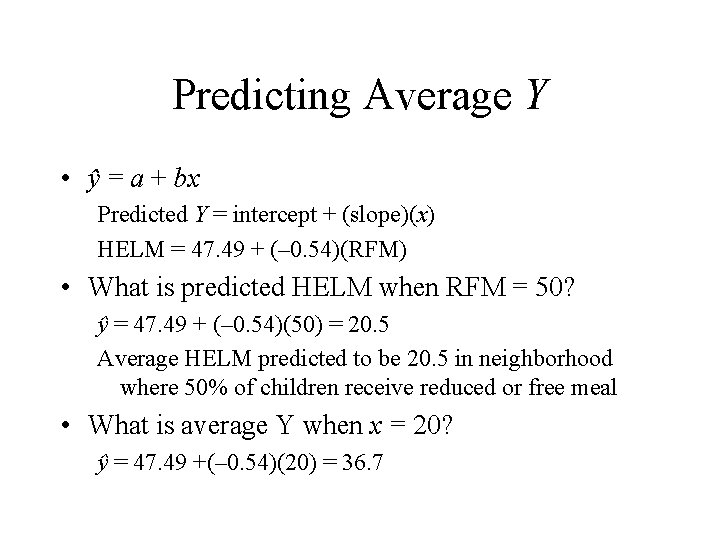
Predicting Average Y • ŷ = a + bx Predicted Y = intercept + (slope)(x) HELM = 47. 49 + (– 0. 54)(RFM) • What is predicted HELM when RFM = 50? ŷ = 47. 49 + (– 0. 54)(50) = 20. 5 Average HELM predicted to be 20. 5 in neighborhood where 50% of children receive reduced or free meal • What is average Y when x = 20? ŷ = 47. 49 +(– 0. 54)(20) = 36. 7

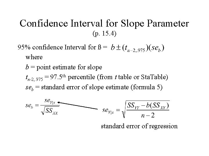
Confidence Interval for Slope Parameter (p. 15. 4) 95% confidence Interval for ß = where b = point estimate for slope tn-2, . 975 = 97. 5 th percentile (from t table or Sta. Table) seb = standard error of slope estimate (formula 5) standard error of regression

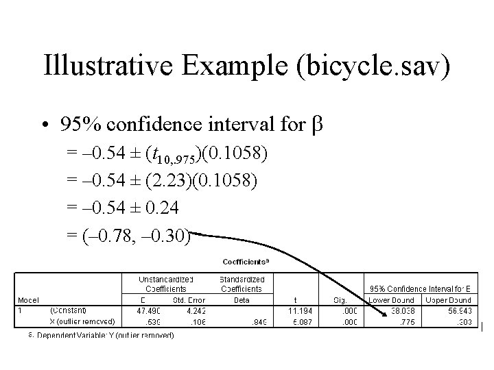
Illustrative Example (bicycle. sav) • 95% confidence interval for = – 0. 54 ± (t 10, . 975)(0. 1058) = – 0. 54 ± (2. 23)(0. 1058) = – 0. 54 ± 0. 24 = (– 0. 78, – 0. 30)

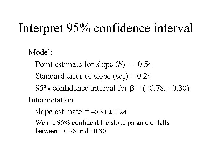
Interpret 95% confidence interval Model: Point estimate for slope (b) = – 0. 54 Standard error of slope (seb) = 0. 24 95% confidence interval for = (– 0. 78, – 0. 30) Interpretation: slope estimate = – 0. 54 ± 0. 24 We are 95% confident the slope parameter falls between – 0. 78 and – 0. 30

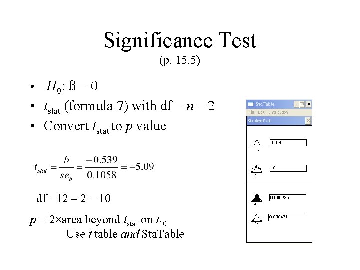
Significance Test (p. 15. 5) • H 0: ß = 0 • tstat (formula 7) with df = n – 2 • Convert tstat to p value df =12 – 2 = 10 p = 2×area beyond tstat on t 10 Use t table and Sta. Table

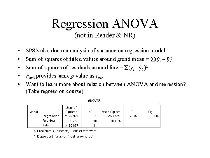
Regression ANOVA (not in Reader & NR) • • • SPSS also does an analysis of variance on regression model Sum of squares of fitted values around grand mean = (ŷi – ÿ)² Sum of squares of residuals around line = (yi– ŷi )² Fstat provides same p value as tstat Want to learn more about relation between ANOVA and regression? (Take regression course)

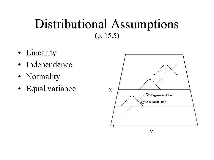
Distributional Assumptions (p. 15. 5) • • Linearity Independence Normality Equal variance

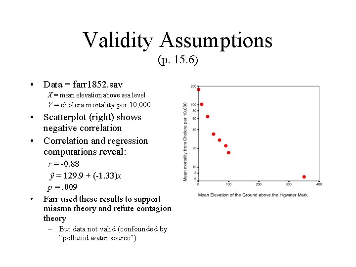
Validity Assumptions (p. 15. 6) • Data = farr 1852. sav X = mean elevation above sea level Y = cholera mortality per 10, 000 • Scatterplot (right) shows negative correlation • Correlation and regression computations reveal: • r = -0. 88 ŷ = 129. 9 + (-1. 33)x p =. 009 Farr used these results to support miasma theory and refute contagion theory – But data not valid (confounded by “polluted water source”)