15 DistributionFree Procedures Copyright Cengage Learning All rights

15. 2 The Wilcoxon Rank-Sum Test Copyright © Cengage Learning. All rights reserved.

The Wilcoxon Rank-Sum Test The two-sample t test is based on the assumption that both population distributions are normal. There are situations, though, in which an investigator would want to use a test that is valid even if the underlying distributions are quite nonnormal. We now describe such a test, called the Wilcoxon rank-sum test. An alternative name for the procedure is the Mann-Whitney test, though the Mann-Whitney test statistic is sometimes expressed in a slightly different form from that of the Wilcoxon test. 3

The Wilcoxon Rank-Sum Test The Wilcoxon test procedure is distribution-free because it will have the desired level of significance for a very large class of underlying distributions. 4

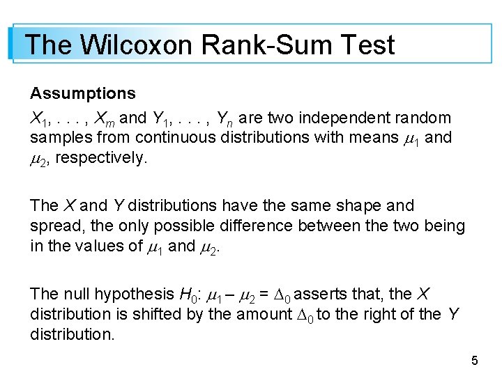
The Wilcoxon Rank-Sum Test Assumptions X 1, . . . , Xm and Y 1, . . . , Yn are two independent random samples from continuous distributions with means 1 and 2, respectively. The X and Y distributions have the same shape and spread, the only possible difference between the two being in the values of 1 and 2. The null hypothesis H 0: 1 – 2 = 0 asserts that, the X distribution is shifted by the amount 0 to the right of the Y distribution. 5

Development of the Test When m = 3, n = 4 6

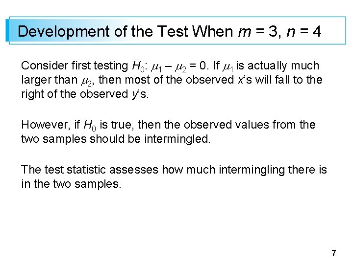
Development of the Test When m = 3, n = 4 Consider first testing H 0: 1 – 2 = 0. If 1 is actually much larger than 2, then most of the observed x’s will fall to the right of the observed y’s. However, if H 0 is true, then the observed values from the two samples should be intermingled. The test statistic assesses how much intermingling there is in the two samples. 7

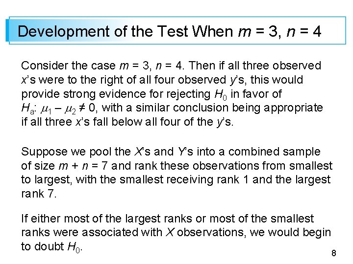
Development of the Test When m = 3, n = 4 Consider the case m = 3, n = 4. Then if all three observed x’s were to the right of all four observed y’s, this would provide strong evidence for rejecting H 0 in favor of Ha: 1 – 2 ≠ 0, with a similar conclusion being appropriate if all three x’s fall below all four of the y’s. Suppose we pool the X’s and Y’s into a combined sample of size m + n = 7 and rank these observations from smallest to largest, with the smallest receiving rank 1 and the largest rank 7. If either most of the largest ranks or most of the smallest ranks were associated with X observations, we would begin to doubt H 0. 8

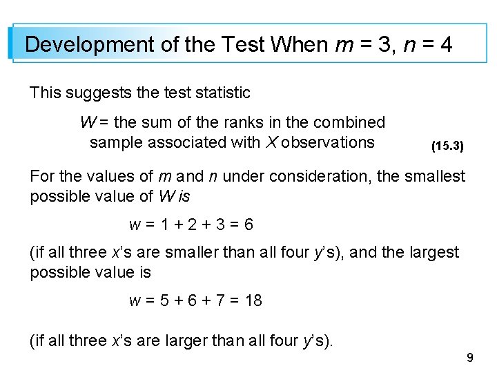
Development of the Test When m = 3, n = 4 This suggests the test statistic W = the sum of the ranks in the combined sample associated with X observations (15. 3) For the values of m and n under consideration, the smallest possible value of W is w=1+2+3=6 (if all three x’s are smaller than all four y’s), and the largest possible value is w = 5 + 6 + 7 = 18 (if all three x’s are larger than all four y’s). 9

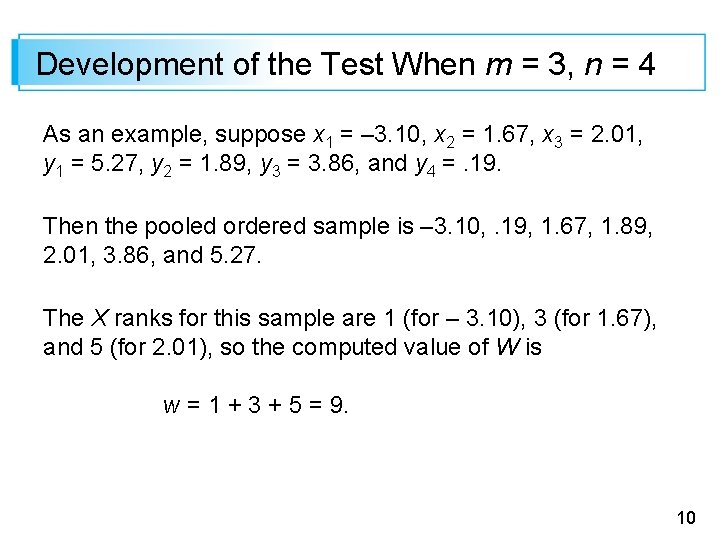
Development of the Test When m = 3, n = 4 As an example, suppose x 1 = – 3. 10, x 2 = 1. 67, x 3 = 2. 01, y 1 = 5. 27, y 2 = 1. 89, y 3 = 3. 86, and y 4 =. 19. Then the pooled ordered sample is – 3. 10, . 19, 1. 67, 1. 89, 2. 01, 3. 86, and 5. 27. The X ranks for this sample are 1 (for – 3. 10), 3 (for 1. 67), and 5 (for 2. 01), so the computed value of W is w = 1 + 3 + 5 = 9. 10

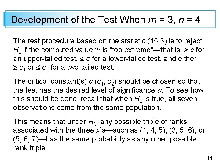
Development of the Test When m = 3, n = 4 The test procedure based on the statistic (15. 3) is to reject H 0 if the computed value w is “too extreme”—that is, c for an upper-tailed test, c for a lower-tailed test, and either c 1 or c 2 for a two-tailed test. The critical constant(s) c (c 1, c 2) should be chosen so that the test has the desired level of significance . To see how this should be done, recall that when H 0 is true, all seven observations come from the same population. This means that under H 0, any possible triple of ranks associated with the three x’s—such as (1, 4, 5), (3, 5, 6), or (5, 6, 7)—has the same probability as any other possible rank triple. 11

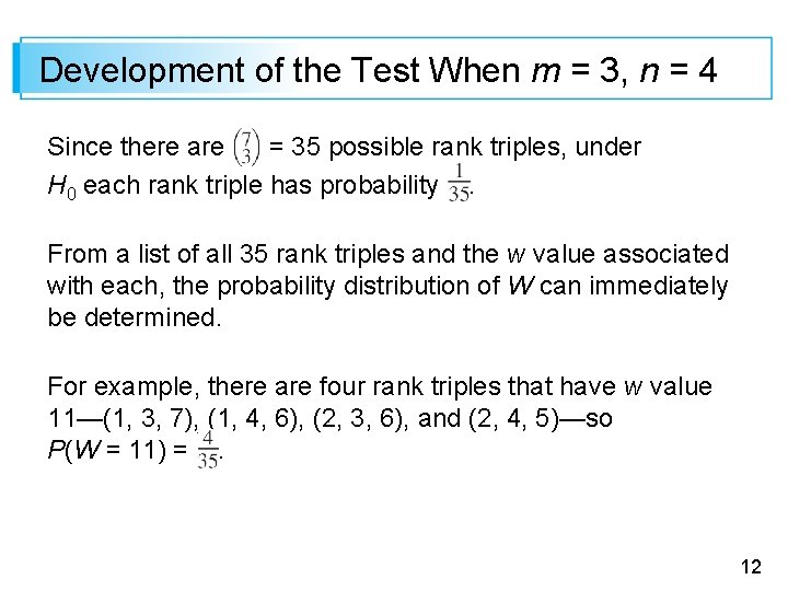
Development of the Test When m = 3, n = 4 Since there are = 35 possible rank triples, under H 0 each rank triple has probability. From a list of all 35 rank triples and the w value associated with each, the probability distribution of W can immediately be determined. For example, there are four rank triples that have w value 11—(1, 3, 7), (1, 4, 6), (2, 3, 6), and (2, 4, 5)—so P(W = 11) =. 12

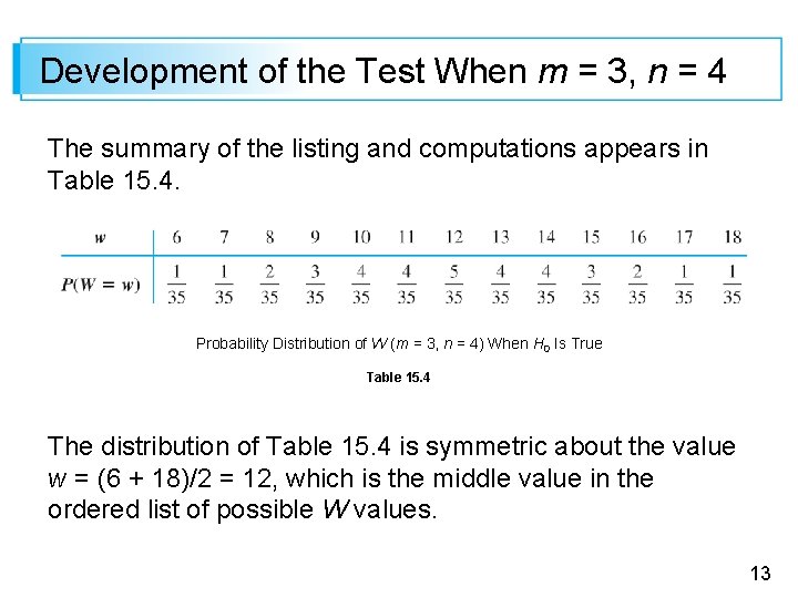
Development of the Test When m = 3, n = 4 The summary of the listing and computations appears in Table 15. 4. Probability Distribution of W (m = 3, n = 4) When H 0 Is True Table 15. 4 The distribution of Table 15. 4 is symmetric about the value w = (6 + 18)/2 = 12, which is the middle value in the ordered list of possible W values. 13

Development of the Test When m = 3, n = 4 This is because the two rank triples (r, s, t) (with r < s < t) and (8 – t, 8 – s, 8 – r) have values of w symmetric about 12, so for each triple with w value below 12, there is a triple with w value above 12 by the same amount. If the alternative hypothesis is Ha: 1 – 2 > 0, then H 0 should be rejected in favor of Ha for large W values. Choosing as the rejection region the set of W values {17, 18}, = P(type I error) = P(reject H 0 when H 0 is true) = P(W = 17 or 18 when H 0 true) = =. 057; the region {17, 18} therefore specifies a test with level of significance approximately. 05. 14

Development of the Test When m = 3, n = 4 Similarly, the region {6, 7}, which is appropriate for Ha: 1 – 2 < 0, has =. 057 . 05. The region {6, 7, 18}, which is appropriate for the two-sided alternative, has = =. 114. The W value for the data given several paragraphs previously was w = 9, which is rather close to the middle value 12, so H 0 would not be rejected at any reasonable level for any one of the three Ha’s. 15

General Description of the Test 16

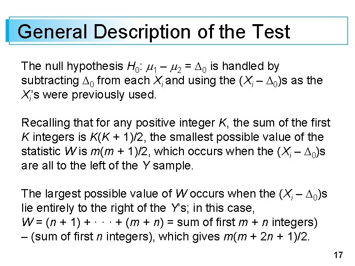
General Description of the Test The null hypothesis H 0: 1 – 2 = 0 is handled by subtracting 0 from each Xi and using the (Xi – 0)s as the Xi’s were previously used. Recalling that for any positive integer K, the sum of the first K integers is K(K + 1)/2, the smallest possible value of the statistic W is m(m + 1)/2, which occurs when the (Xi – 0)s are all to the left of the Y sample. The largest possible value of W occurs when the (Xi – 0)s lie entirely to the right of the Y’s; in this case, W = (n + 1) + · · · + (m + n) = sum of first m + n integers) – (sum of first n integers), which gives m(m + 2 n + 1)/2. 17

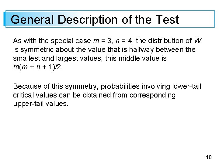
General Description of the Test As with the special case m = 3, n = 4, the distribution of W is symmetric about the value that is halfway between the smallest and largest values; this middle value is m(m + n + 1)/2. Because of this symmetry, probabilities involving lower-tail critical values can be obtained from corresponding upper-tail values. 18

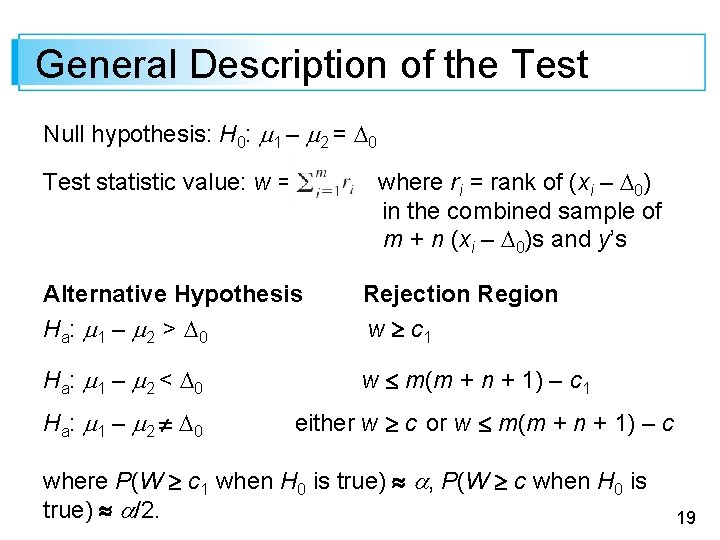
General Description of the Test Null hypothesis: H 0: 1 – 2 = 0 where ri = rank of (xi – 0) in the combined sample of m + n (xi – 0)s and y’s Test statistic value: w = Alternative Hypothesis H a: 1 – 2 > 0 Rejection Region w c 1 H a: 1 – 2 < 0 w m(m + n + 1) – c 1 H a: 1 – 2 0 either w c or w m(m + n + 1) – c where P(W c 1 when H 0 is true) , P(W c when H 0 is true) /2. 19

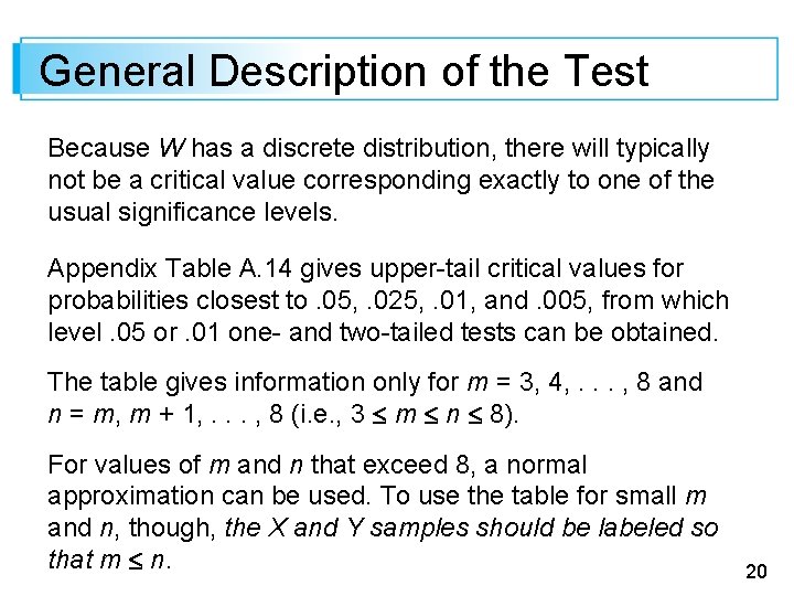
General Description of the Test Because W has a discrete distribution, there will typically not be a critical value corresponding exactly to one of the usual significance levels. Appendix Table A. 14 gives upper-tail critical values for probabilities closest to. 05, . 025, . 01, and. 005, from which level. 05 or. 01 one- and two-tailed tests can be obtained. The table gives information only for m = 3, 4, . . . , 8 and n = m, m + 1, . . . , 8 (i. e. , 3 m n 8). For values of m and n that exceed 8, a normal approximation can be used. To use the table for small m and n, though, the X and Y samples should be labeled so that m n. 20

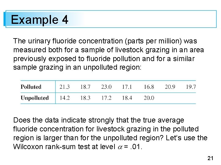
Example 4 The urinary fluoride concentration (parts per million) was measured both for a sample of livestock grazing in an area previously exposed to fluoride pollution and for a similar sample grazing in an unpolluted region: Does the data indicate strongly that the true average fluoride concentration for livestock grazing in the polluted region is larger than for the unpolluted region? Let’s use the Wilcoxon rank-sum test at level =. 01. 21

Example 4 cont’d The sample sizes here are 7 and 5. To obtain m n, label the unpolluted observations as the x’s (x 1 = 14. 2, . . . , x 5 = 20. 0). Thus 1 is the true average fluoride concentration without pollution, and 2 is the true average concentration with pollution. The alternative hypothesis is Ha: 1 – 2 < 0 (pollution is associated with an increase in concentration), so a lower-tailed test is appropriate. 22

Example 4 cont’d From Appendix Table A. 14 with m = 5 and n = 7, P(W 47 when H 0 is true) . 01. The critical value for the lower-tailed test is therefore m(m + n + 1) – 47 = 5(13) – 47 = 18; H 0 will now be rejected if w 18. 23

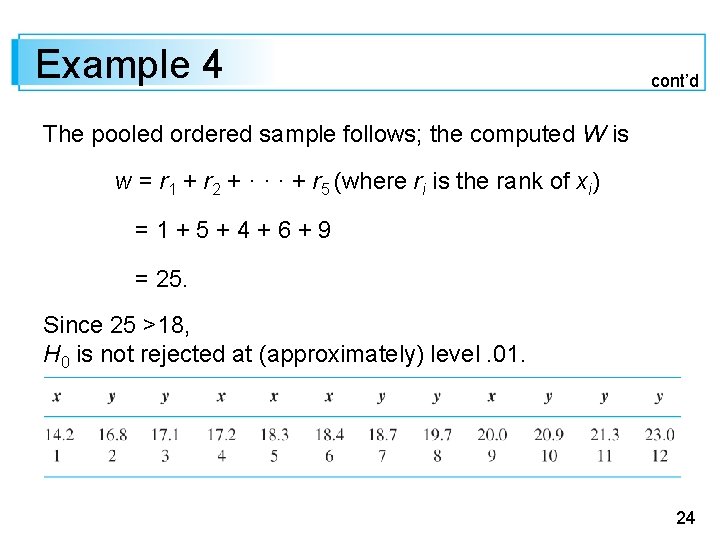
Example 4 cont’d The pooled ordered sample follows; the computed W is w = r 1 + r 2 + · · · + r 5 (where ri is the rank of xi) =1+5+4+6+9 = 25. Since 25 >18, H 0 is not rejected at (approximately) level. 01. 24

A Normal Approximation for W 25

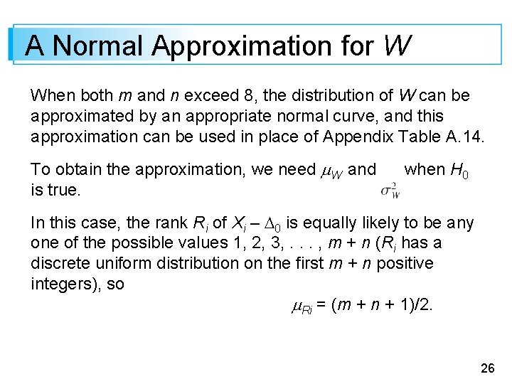
A Normal Approximation for W When both m and n exceed 8, the distribution of W can be approximated by an appropriate normal curve, and this approximation can be used in place of Appendix Table A. 14. To obtain the approximation, we need W and is true. when H 0 In this case, the rank Ri of Xi – 0 is equally likely to be any one of the possible values 1, 2, 3, . . . , m + n (Ri has a discrete uniform distribution on the first m + n positive integers), so Ri = (m + n + 1)/2. 26

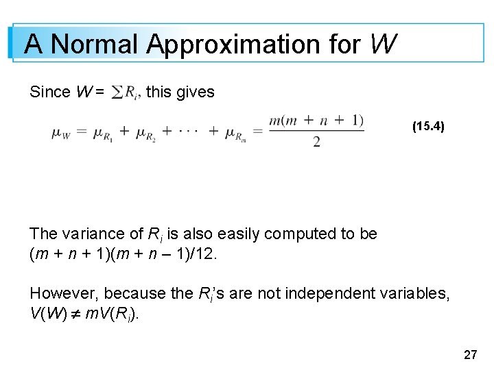
A Normal Approximation for W Since W = this gives (15. 4) The variance of Ri is also easily computed to be (m + n + 1)(m + n – 1)/12. However, because the Ri’s are not independent variables, V(W) m. V(Ri). 27

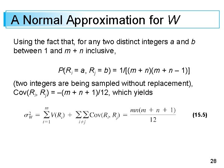
A Normal Approximation for W Using the fact that, for any two distinct integers a and b between 1 and m + n inclusive, P(Ri = a, Rj = b) = 1/[(m + n)(m + n – 1)] (two integers are being sampled without replacement), Cov(Ri, Rj) = –(m + n + 1)/12, which yields (15. 5) 28

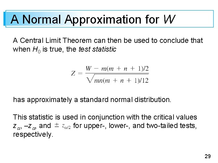
A Normal Approximation for W A Central Limit Theorem can then be used to conclude that when H 0 is true, the test statistic has approximately a standard normal distribution. This statistic is used in conjunction with the critical values z , –z , and for upper-, lower-, and two-tailed tests, respectively. 29

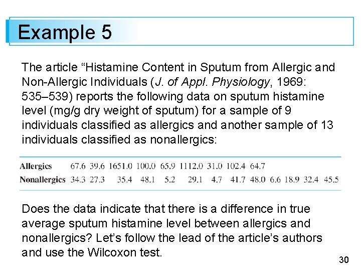
Example 5 The article “Histamine Content in Sputum from Allergic and Non-Allergic Individuals (J. of Appl. Physiology, 1969: 535– 539) reports the following data on sputum histamine level (mg/g dry weight of sputum) for a sample of 9 individuals classified as allergics and another sample of 13 individuals classified as nonallergics: Does the data indicate that there is a difference in true average sputum histamine level between allergics and nonallergics? Let’s follow the lead of the article’s authors and use the Wilcoxon test. 30

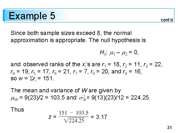
Example 5 cont’d Since both sample sizes exceed 8, the normal approximation is appropriate. The null hypothesis is H 0: 1 – 2 = 0, and observed ranks of the xi’s are r 1 = 18, r 2 = 11, r 3 = 22, r 4 = 19, r 5 = 17, r 6 = 21, r 7 = 7, r 8 = 20, and r 9 = 16, so w = ri = 151. The mean and variance of W are given by W = 9(23)/2 = 103. 5 and = 9(13)(23)/12 = 224. 25. Thus z= = 3. 17 31

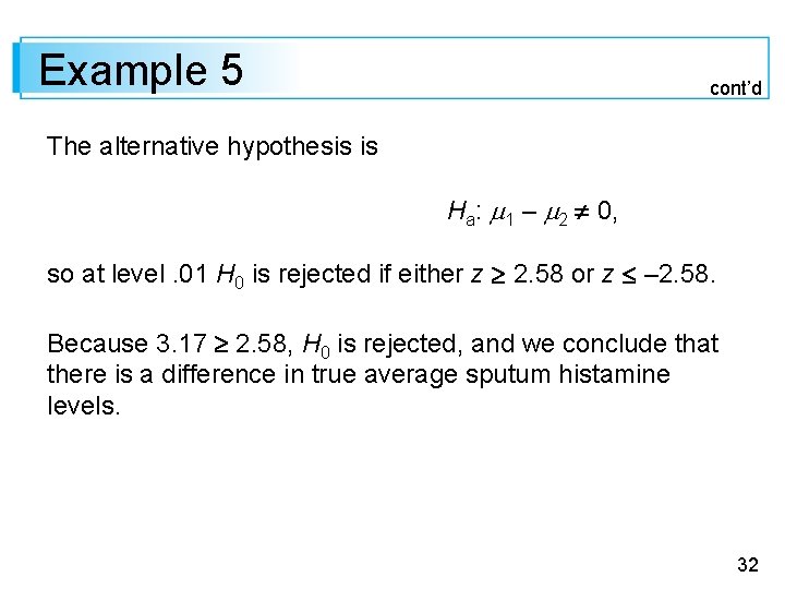
Example 5 cont’d The alternative hypothesis is Ha: 1 – 2 0, so at level. 01 H 0 is rejected if either z 2. 58 or z – 2. 58. Because 3. 17 2. 58, H 0 is rejected, and we conclude that there is a difference in true average sputum histamine levels. 32

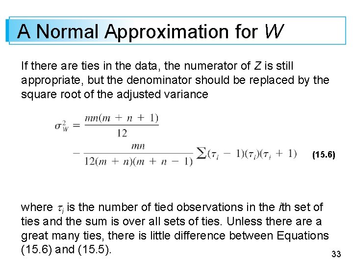
A Normal Approximation for W If there are ties in the data, the numerator of Z is still appropriate, but the denominator should be replaced by the square root of the adjusted variance (15. 6) where ti is the number of tied observations in the ith set of ties and the sum is over all sets of ties. Unless there a great many ties, there is little difference between Equations (15. 6) and (15. 5). 33

Efficiency of the Wilcoxon Rank-Sum Test 34

Efficiency of the Wilcoxon Rank-Sum Test When the distributions being sampled are both normal with 1 = 2, and therefore have the same shapes and spreads, either the pooled t test or the Wilcoxon test can be used (the two-sample t test assumes normality but not equal variances, so assumptions underlying its use are more restrictive in one sense and less in another than those for Wilcoxon’s test). In this situation, the pooled t test is best among all possible tests in the sense of minimizing for any fixed . However, an investigator can never be absolutely certain that underlying assumptions are satisfied. 35

Efficiency of the Wilcoxon Rank-Sum Test It is therefore relevant to ask (1) how much is lost by using Wilcoxon’s test rather than the pooled t test when the distributions are normal with equal variances and (2) how W compares to T in nonnormal situations. The notion of test efficiency was discussed in the previous section in connection with the one-sample t test and Wilcoxon signed-rank test. The results for the two-sample tests are the same as those for the one-sample tests. 36

Efficiency of the Wilcoxon Rank-Sum Test When normality and equal variances both hold, the rank-sum test is approximately 95% as efficient as the pooled t test in large samples. That is, the t test will give the same error probabilities as the Wilcoxon test using slightly smaller sample sizes. On the other hand, the Wilcoxon test will always be at least 86% as efficient as the pooled t test and may be much more efficient if the underlying distributions are very nonnormal, especially with heavy tails. 37

Efficiency of the Wilcoxon Rank-Sum Test The comparison of the Wilcoxon test with the two-sample (unpooled) t test is less clear-cut. The t test is not known to be the best test in any sense, so it seems safe to conclude that as long as the population distributions have similar shapes and spreads, the behavior of the Wilcoxon test should compare quite favorably to the two-sample t test. Lastly, we note that calculations for the Wilcoxon test are quite difficult. 38

Efficiency of the Wilcoxon Rank-Sum Test This is because the distribution of W when H 0 is false depends not only on 1 – 2 but also on the shapes of the two distributions. For most underlying distributions, the nonnull distribution of W is virtually intractable. This is why statisticians have developed large-sample (asymptotic relative) efficiency as a means of comparing tests. With the capabilities of modern-day computer software, another approach to calculation of is to carry out a simulation experiment. 39