15 853 Algorithms in the Real World Linear

15 -853: Algorithms in the Real World Linear and Integer Programming I – Introduction – Geometric Interpretation – Simplex Method 15 -853 Page 1

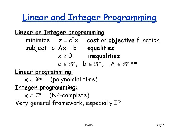
Linear and Integer Programming Linear or Integer programming minimize z c. Tx cost or objective function subject to Ax b equalities x 0 inequalities c n, b m , A n x m Linear programming: x n (polynomial time) Integer programming: x n (NP-complete) Very general framework, especially IP 15 -853 Page 2

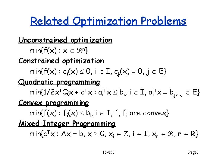
Related Optimization Problems Unconstrained optimization min{f(x) : x n} Constrained optimization min{f(x) : ci(x) 0, i I, cj(x) 0, j E} Quadratic programming min{1/2 x. TQx + c. Tx : ai. Tx bi, i I, ai. Tx bj, j E} Convex programming min{f(x) : fi(x) bi, i I, f, fi are convex} Mixed Integer Programming min{c. Tx : Ax b, x 0, xi , i I, xr , r R} 15 -853 Page 3

How important is optimization? • • • 50+ packages available 1300+ papers just on interior-point methods 100+ books in the library 10+ courses at most Universities 100 s of companies All major airlines, delivery companies, trucking companies, manufacturers, … make serious use of optimization. 15 -853 Page 4

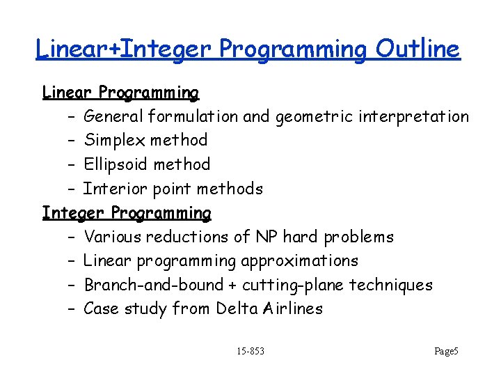
Linear+Integer Programming Outline Linear Programming – General formulation and geometric interpretation – Simplex method – Ellipsoid method – Interior point methods Integer Programming – Various reductions of NP hard problems – Linear programming approximations – Branch-and-bound + cutting-plane techniques – Case study from Delta Airlines 15 -853 Page 5

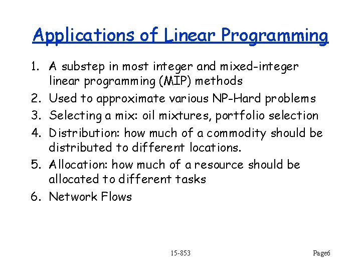
Applications of Linear Programming 1. A substep in most integer and mixed-integer linear programming (MIP) methods 2. Used to approximate various NP-Hard problems 3. Selecting a mix: oil mixtures, portfolio selection 4. Distribution: how much of a commodity should be distributed to different locations. 5. Allocation: how much of a resource should be allocated to different tasks 6. Network Flows 15 -853 Page 6

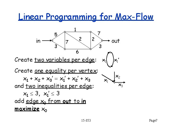
Linear Programming for Max-Flow in 1 5 3 2 7 3 6 Create two variables per edge: x 1 Create one equality per vertex: x 1 + x 2 + x 3 ’ x 1’ + x 2 ’ + x 3 x 1 and two inequalities per edge: x 1 3, x 1’ 3 add edge x 0 from out to in maximize x 0 15 -853 out x 1 ’ x 2 x 3 Page 7

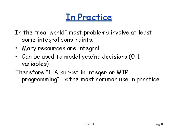
In Practice In the “real world” most problems involve at least some integral constraints. • Many resources are integral • Can be used to model yes/no decisions (0 -1 variables) Therefore “ 1. A subset in integer or MIP programming” is the most common use in practice 15 -853 Page 8

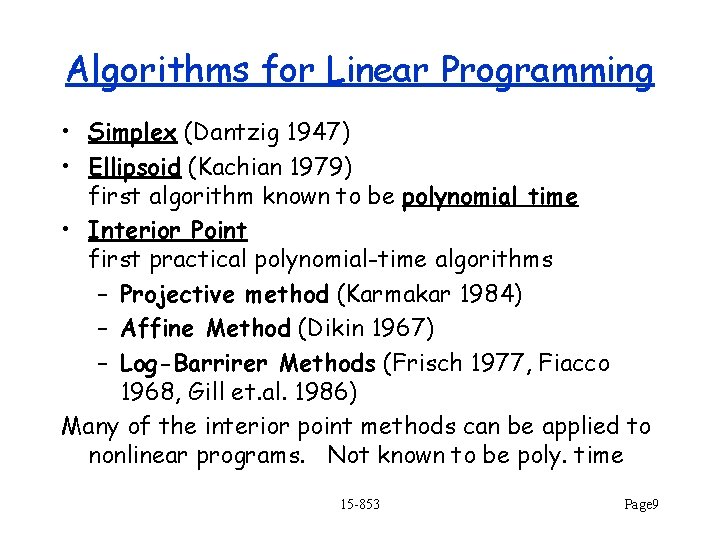
Algorithms for Linear Programming • Simplex (Dantzig 1947) • Ellipsoid (Kachian 1979) first algorithm known to be polynomial time • Interior Point first practical polynomial-time algorithms – Projective method (Karmakar 1984) – Affine Method (Dikin 1967) – Log-Barrirer Methods (Frisch 1977, Fiacco 1968, Gill et. al. 1986) Many of the interior point methods can be applied to nonlinear programs. Not known to be poly. time 15 -853 Page 9

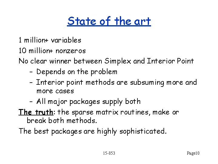
State of the art 1 million+ variables 10 million+ nonzeros No clear winner between Simplex and Interior Point – Depends on the problem – Interior point methods are subsuming more and more cases – All major packages supply both The truth: the sparse matrix routines, make or break both methods. The best packages are highly sophisticated. 15 -853 Page 10

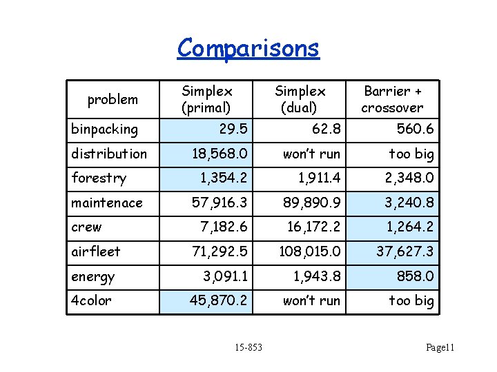
Comparisons problem binpacking Simplex (primal) Simplex (dual) Barrier + crossover 29. 5 62. 8 560. 6 18, 568. 0 won’t run too big 1, 354. 2 1, 911. 4 2, 348. 0 57, 916. 3 89, 890. 9 3, 240. 8 7, 182. 6 16, 172. 2 1, 264. 2 71, 292. 5 108, 015. 0 37, 627. 3 energy 3, 091. 1 1, 943. 8 858. 0 4 color 45, 870. 2 won’t run too big distribution forestry maintenace crew airfleet 15 -853 Page 11

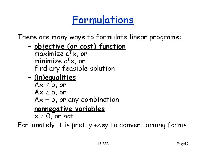
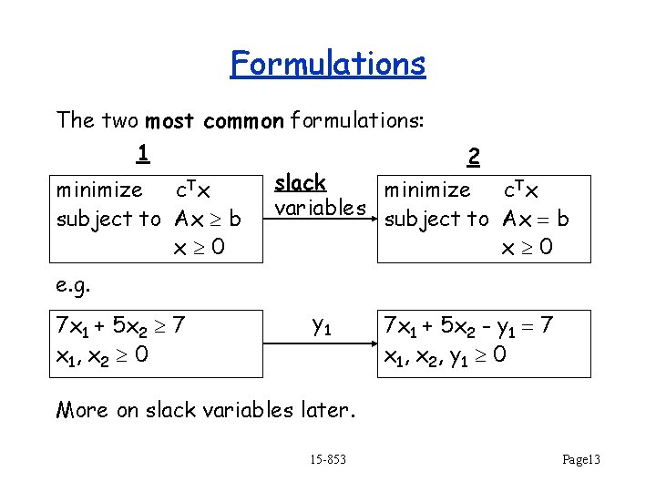
Formulations There are many ways to formulate linear programs: – objective (or cost) function maximize c. Tx, or minimize c. Tx, or find any feasible solution – (in)equalities Ax b, or any combination – nonnegative variables x 0, or not Fortunately it is pretty easy to convert among forms 15 -853 Page 12

Formulations The two most common formulations: 1 minimize c. Tx subject to Ax b x 0 2 slack minimize c. Tx variables subject to Ax b x 0 e. g. 7 x 1 + 5 x 2 7 x 1, x 2 0 y 1 7 x 1 + 5 x 2 - y 1 7 x 1, x 2 , y 1 0 More on slack variables later. 15 -853 Page 13

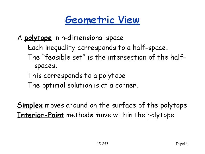
Geometric View A polytope in n-dimensional space Each inequality corresponds to a half-space. The “feasible set” is the intersection of the halfspaces. This corresponds to a polytope The optimal solution is at a corner. Simplex moves around on the surface of the polytope Interior-Point methods move within the polytope 15 -853 Page 14

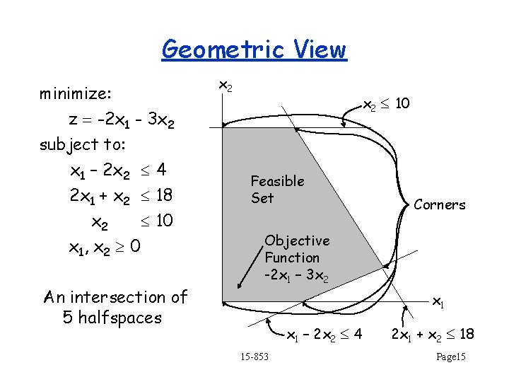
Geometric View minimize: z -2 x 1 - 3 x 2 subject to: x 1 – 2 x 2 4 2 x 1 + x 2 18 x 2 10 x 1, x 2 0 An intersection of 5 halfspaces x 2 10 Feasible Set Corners Objective Function -2 x 1 – 3 x 2 x 1 – 2 x 2 4 15 -853 2 x 1 + x 2 18 Page 15

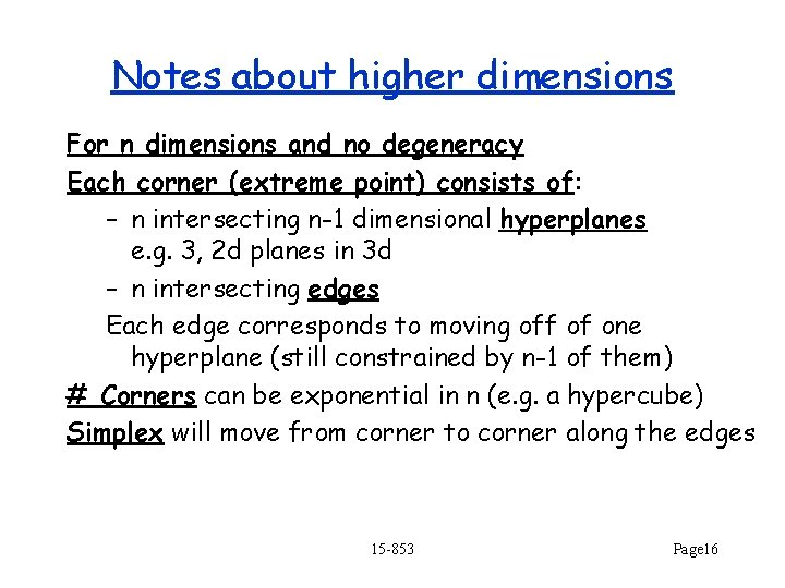
Notes about higher dimensions For n dimensions and no degeneracy Each corner (extreme point) consists of: – n intersecting n-1 dimensional hyperplanes e. g. 3, 2 d planes in 3 d – n intersecting edges Each edge corresponds to moving off of one hyperplane (still constrained by n-1 of them) # Corners can be exponential in n (e. g. a hypercube) Simplex will move from corner to corner along the edges 15 -853 Page 16

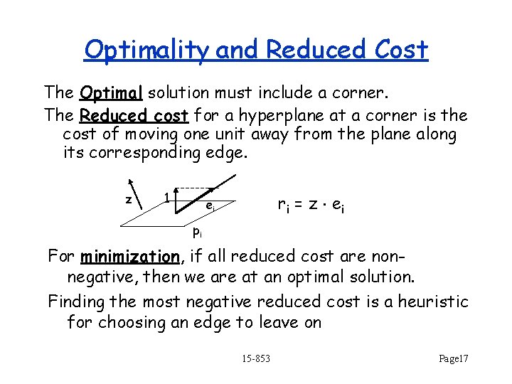
Optimality and Reduced Cost The Optimal solution must include a corner. The Reduced cost for a hyperplane at a corner is the cost of moving one unit away from the plane along its corresponding edge. z 1 ri = z e i ei pi For minimization, if all reduced cost are nonnegative, then we are at an optimal solution. Finding the most negative reduced cost is a heuristic for choosing an edge to leave on 15 -853 Page 17

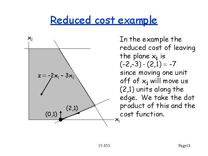
Reduced cost example x 2 In the example the reduced cost of leaving the plane x 1 is (-2, -3) (2, 1) -7 since moving one unit off of x 1 will move us (2, 1) units along the edge. We take the dot product of this and the cost function. z -2 x 1 – 3 x 2 (0, 1) (2, 1) x 1 15 -853 Page 18

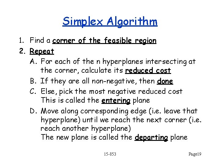
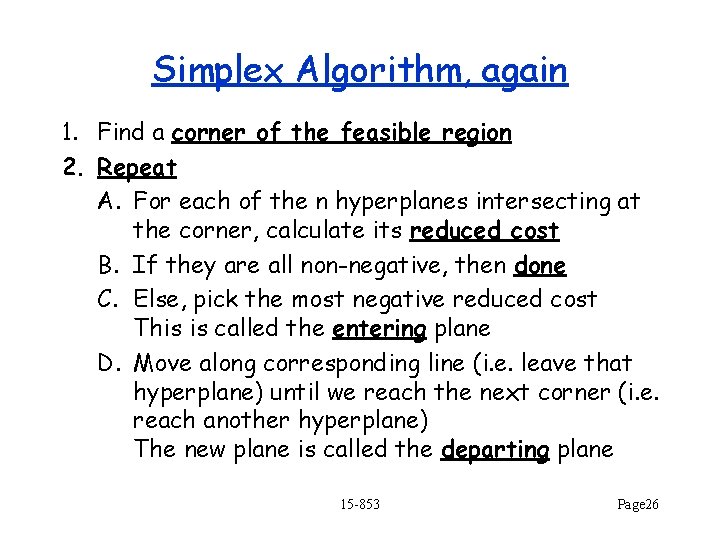
Simplex Algorithm 1. Find a corner of the feasible region 2. Repeat A. For each of the n hyperplanes intersecting at the corner, calculate its reduced cost B. If they are all non-negative, then done C. Else, pick the most negative reduced cost This is called the entering plane D. Move along corresponding edge (i. e. leave that hyperplane) until we reach the next corner (i. e. reach another hyperplane) The new plane is called the departing plane 15 -853 Page 19

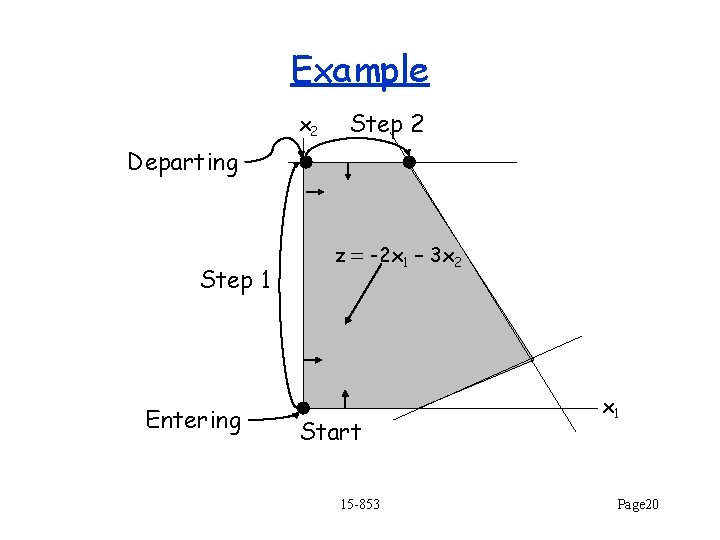
Example x 2 Step 2 Departing Step 1 Entering z -2 x 1 – 3 x 2 Start 15 -853 x 1 Page 20

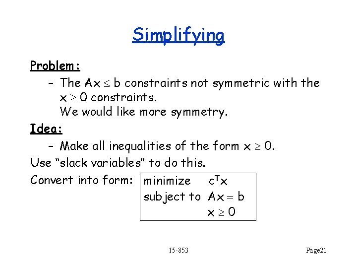
Simplifying Problem: – The Ax b constraints not symmetric with the x 0 constraints. We would like more symmetry. Idea: – Make all inequalities of the form x 0. Use “slack variables” to do this. Convert into form: minimize c. Tx subject to Ax b x 0 15 -853 Page 21

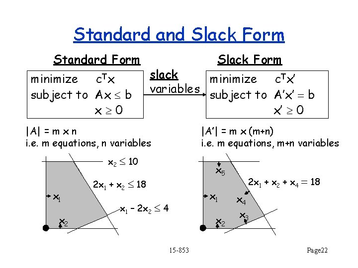
Standard and Slack Form Standard Form minimize c. Tx subject to Ax b x 0 Slack Form slack minimize c. Tx’ variables subject to A’x’ b x’ 0 |A| = m x n i. e. m equations, n variables |A’| = m x (m+n) i. e. m equations, m+n variables x 2 10 x 1 x 2 x 5 2 x 1 + x 2 18 x 1 – 2 x 2 4 x 2 15 -853 2 x 1 + x 2 + x 4 18 x 4 x 3 Page 22

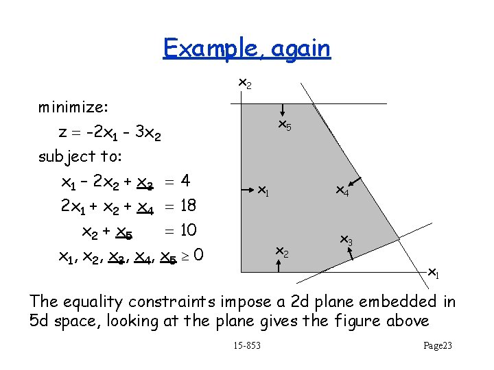
Example, again x 2 minimize: z -2 x 1 - 3 x 2 subject to: x 1 – 2 x 2 + x 3 4 2 x 1 + x 2 + x 4 18 x 2 + x 5 10 x 1, x 2 , x 3 , x 4 , x 5 0 x 5 x 1 x 4 x 2 x 3 x 1 The equality constraints impose a 2 d plane embedded in 5 d space, looking at the plane gives the figure above 15 -853 Page 23

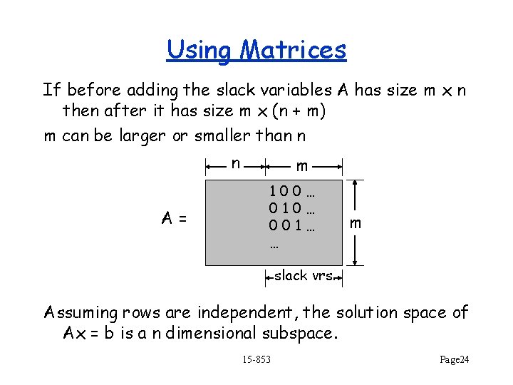
Using Matrices If before adding the slack variables A has size m x n then after it has size m x (n + m) m can be larger or smaller than n n A= m 100… 010… 001… … m slack vrs. Assuming rows are independent, the solution space of Ax = b is a n dimensional subspace. 15 -853 Page 24

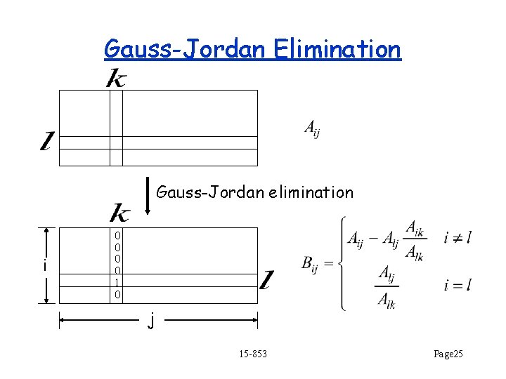
Gauss-Jordan Elimination Gauss-Jordan elimination i 0 0 1 0 j 15 -853 Page 25

Simplex Algorithm, again 1. Find a corner of the feasible region 2. Repeat A. For each of the n hyperplanes intersecting at the corner, calculate its reduced cost B. If they are all non-negative, then done C. Else, pick the most negative reduced cost This is called the entering plane D. Move along corresponding line (i. e. leave that hyperplane) until we reach the next corner (i. e. reach another hyperplane) The new plane is called the departing plane 15 -853 Page 26

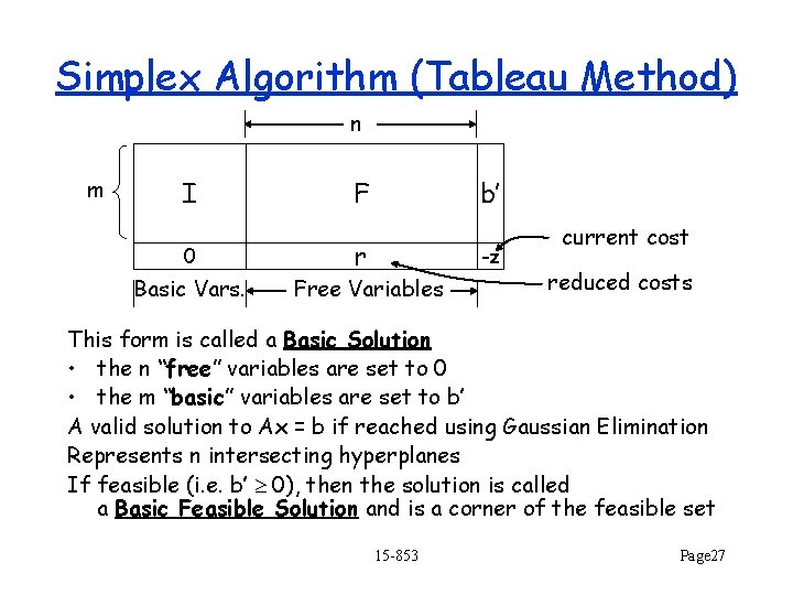
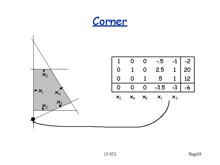
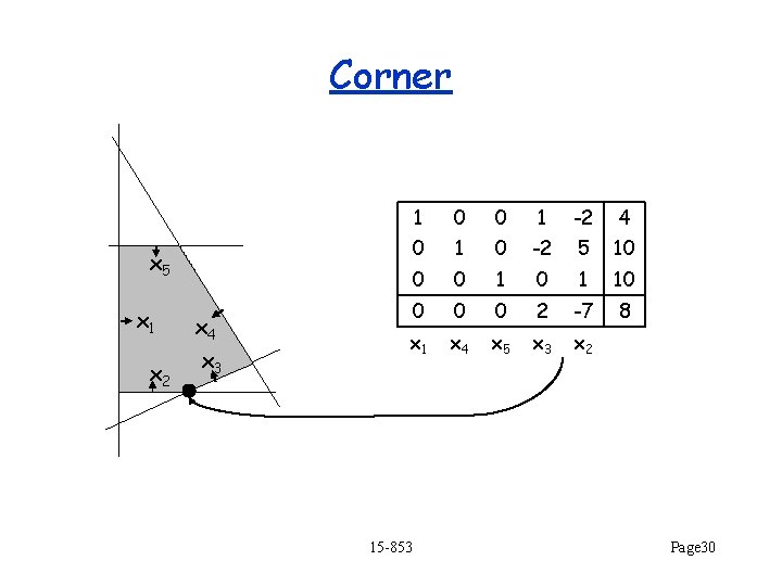
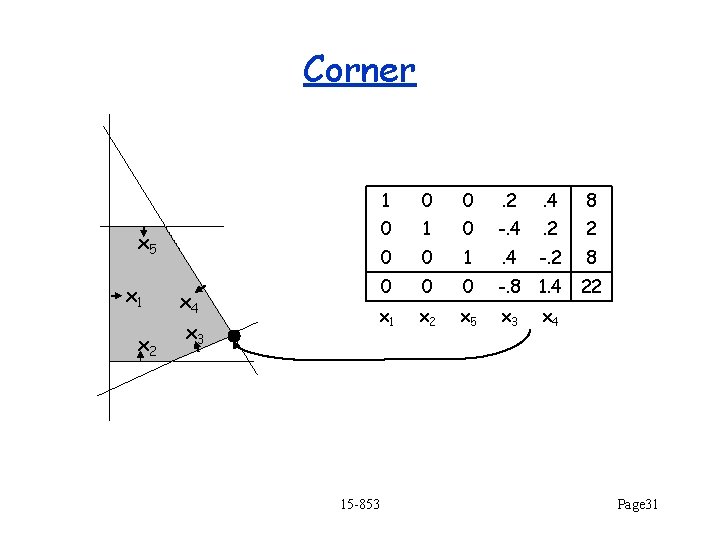
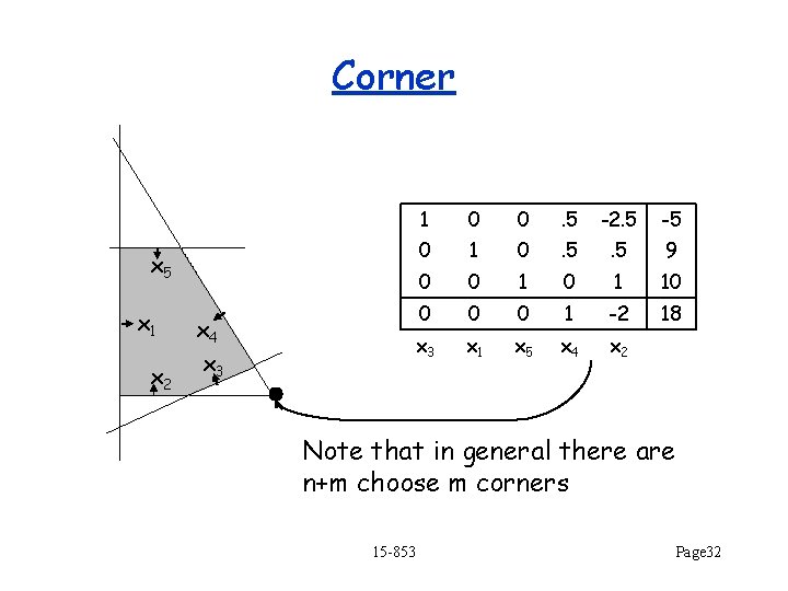
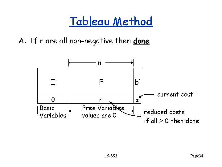
Simplex Algorithm (Tableau Method) n m I 0 Basic Vars. F b’ r -z Free Variables current cost reduced costs This form is called a Basic Solution • the n “free” variables are set to 0 • the m “basic” variables are set to b’ A valid solution to Ax = b if reached using Gaussian Elimination Represents n intersecting hyperplanes If feasible (i. e. b’ 0), then the solution is called a Basic Feasible Solution and is a corner of the feasible set 15 -853 Page 27

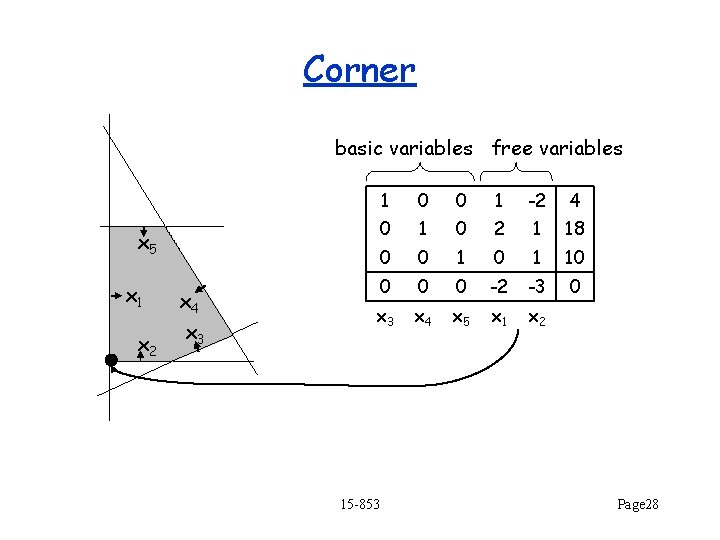
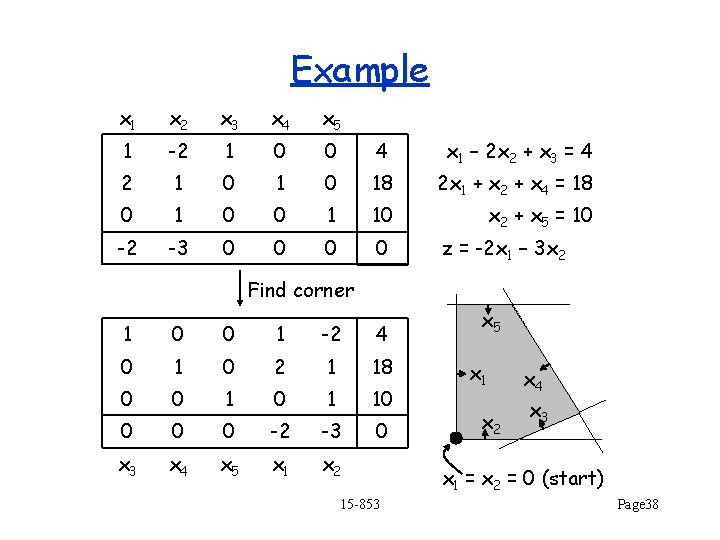
Corner basic variables free variables x 5 x 1 x 2 x 4 x 3 1 0 0 1 -2 4 0 1 0 2 1 18 0 0 1 10 0 -2 -3 0 x 3 x 4 x 5 x 1 x 2 15 -853 Page 28

Corner 1 0 0 -. 5 -1 -2 0 1 0 2. 5 1 20 0 0 1 . 5 1 12 0 0 0 -3. 5 -3 -6 x 2 x 4 x 5 x 1 x 3 x 5 x 1 x 2 x 4 x 3 15 -853 Page 29

Corner x 5 x 1 x 2 x 4 x 3 1 0 0 1 -2 4 0 1 0 -2 5 10 0 0 1 10 0 2 -7 8 x 1 x 4 x 5 x 3 x 2 15 -853 Page 30

Corner 1 0 0 . 2 . 4 8 0 1 0 -. 4 . 2 2 0 0 1 . 4 -. 2 8 0 0 0 -. 8 1. 4 x 1 x 2 x 5 x 3 x 5 x 1 x 2 x 4 x 3 15 -853 22 x 4 Page 31

Corner 1 0 0 . 5 -2. 5 -5 0 1 0 . 5 9 0 0 1 10 0 1 -2 18 x 3 x 1 x 5 x 4 x 2 x 5 x 1 x 2 x 4 x 3 Note that in general there are n+m choose m corners 15 -853 Page 32

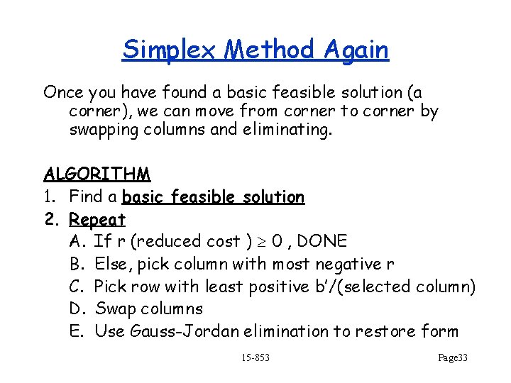
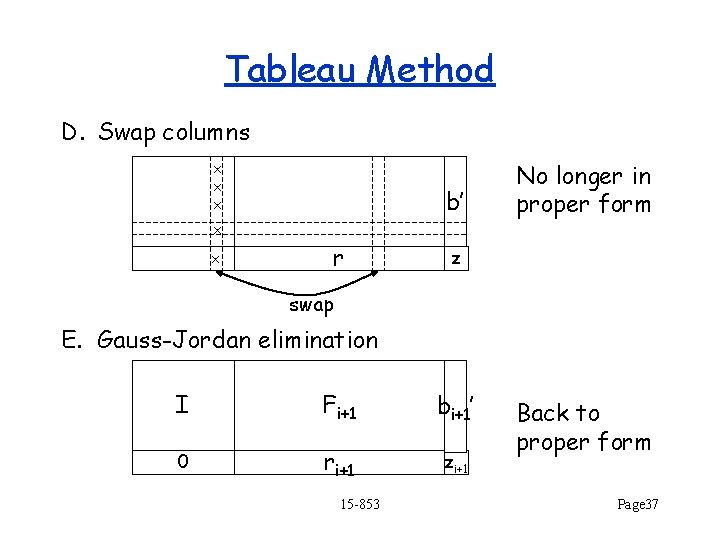
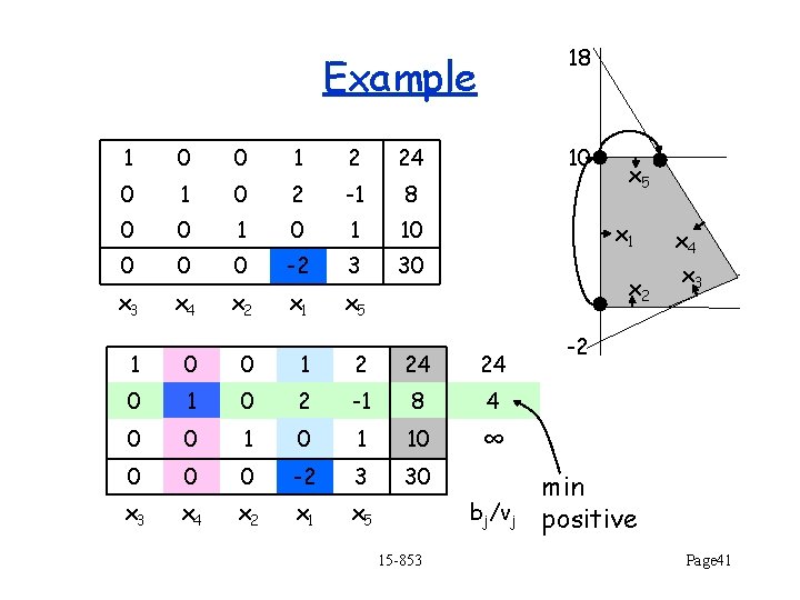
Simplex Method Again Once you have found a basic feasible solution (a corner), we can move from corner to corner by swapping columns and eliminating. ALGORITHM 1. Find a basic feasible solution 2. Repeat A. If r (reduced cost ) 0 , DONE B. Else, pick column with most negative r C. Pick row with least positive b’/(selected column) D. Swap columns E. Use Gauss-Jordan elimination to restore form 15 -853 Page 33

Tableau Method A. If r are all non-negative then done n I 0 Basic Variables F b’ r Free Variables values are 0 15 -853 z current cost reduced costs if all 0 then done Page 34

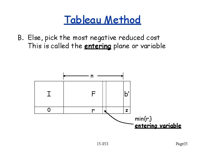
Tableau Method B. Else, pick the most negative reduced cost This is called the entering plane or variable n I F b’ 0 r z min{ri} entering variable 15 -853 Page 35

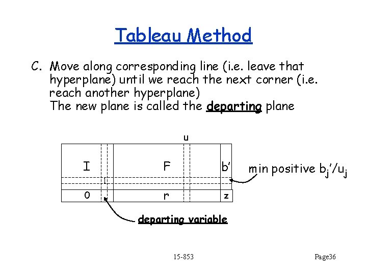
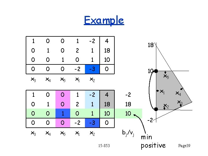
Tableau Method C. Move along corresponding line (i. e. leave that hyperplane) until we reach the next corner (i. e. reach another hyperplane) The new plane is called the departing plane u I F b’ r z 1 0 min positive bj’/uj departing variable 15 -853 Page 36

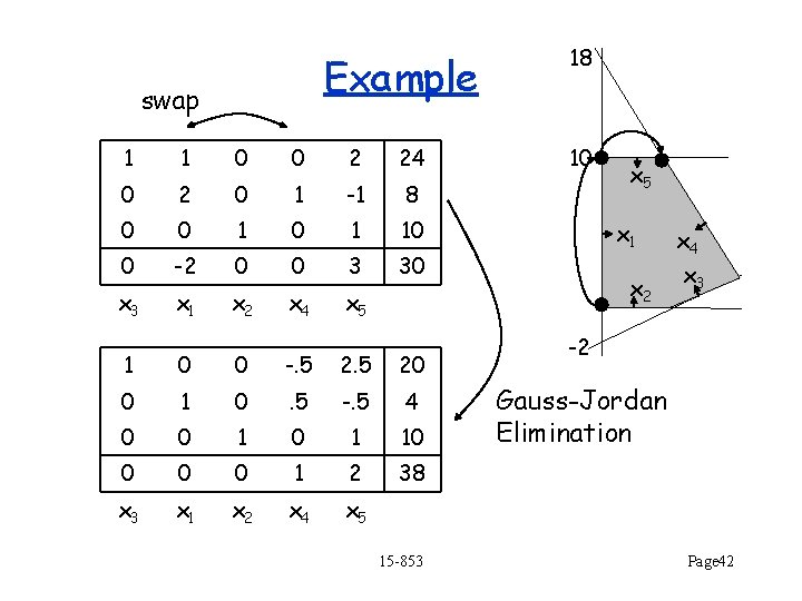
Tableau Method D. Swap columns x x x b’ x x r No longer in proper form z swap E. Gauss-Jordan elimination I Fi+1 bi+1’ 0 ri+1 zi+1 15 -853 Back to proper form Page 37

Example x 1 x 2 x 3 x 4 x 5 1 -2 1 0 0 4 x 1 – 2 x 2 + x 3 = 4 2 1 0 18 2 x 1 + x 2 + x 4 = 18 0 1 0 0 1 10 x 2 + x 5 = 10 -2 -3 0 0 z = -2 x 1 – 3 x 2 Find corner 1 0 0 1 -2 4 0 1 0 2 1 18 0 0 1 10 0 -2 -3 0 x 3 x 4 x 5 x 1 x 2 15 -853 x 5 x 1 x 2 x 4 x 3 x 1 = x 2 = 0 (start) Page 38

Example 1 0 0 1 -2 4 0 1 0 2 1 18 0 0 1 10 0 -2 -3 0 x 3 x 4 x 5 x 1 x 2 1 0 0 1 -2 4 -2 0 1 0 2 1 18 18 0 0 1 10 10 0 -2 -3 0 x 3 x 4 x 5 x 1 x 2 18 10 bj/vj 15 -853 x 5 x 1 x 2 x 4 x 3 -2 min positive Page 39

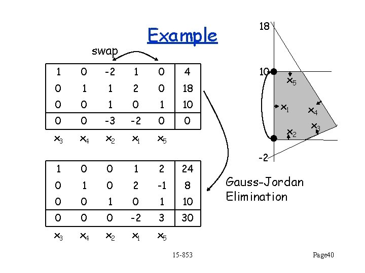
Example swap 1 0 -2 1 0 4 0 1 1 2 0 18 0 0 1 10 0 0 -3 -2 0 0 x 3 x 4 x 2 x 1 x 5 1 0 0 1 2 24 0 1 0 2 -1 8 0 0 1 10 0 -2 3 30 x 3 x 4 x 2 x 1 x 5 15 -853 18 10 x 5 x 1 x 2 x 4 x 3 -2 Gauss-Jordan Elimination Page 40

18 Example 1 0 0 1 2 24 0 1 0 2 -1 8 0 0 1 10 0 -2 3 30 x 3 x 4 x 2 x 1 x 5 10 x 1 x 2 1 0 0 1 2 24 24 0 1 0 2 -1 8 4 0 0 1 10 ∞ 0 0 0 -2 3 30 x 3 x 4 x 2 x 1 x 5 bj/vj 15 -853 x 5 x 4 x 3 -2 min positive Page 41

Example swap 1 1 0 0 2 24 0 2 0 1 -1 8 0 0 1 10 0 -2 0 0 3 30 x 3 x 1 x 2 x 4 x 5 1 0 0 -. 5 20 0 1 0 . 5 -. 5 4 0 0 1 10 0 1 2 38 x 3 x 1 x 2 x 4 x 5 15 -853 18 10 x 5 x 1 x 2 x 4 x 3 -2 Gauss-Jordan Elimination Page 42

Simplex Concluding remarks For dense matrices, takes O(n(n+m)) time per iteration Can take an exponential number of iterations. In practice, sparse methods are used for the iterations. 15 -853 Page 43

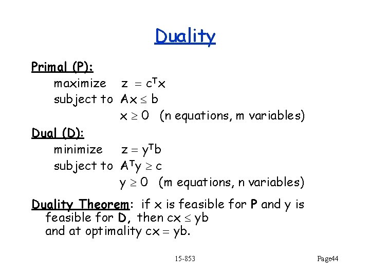
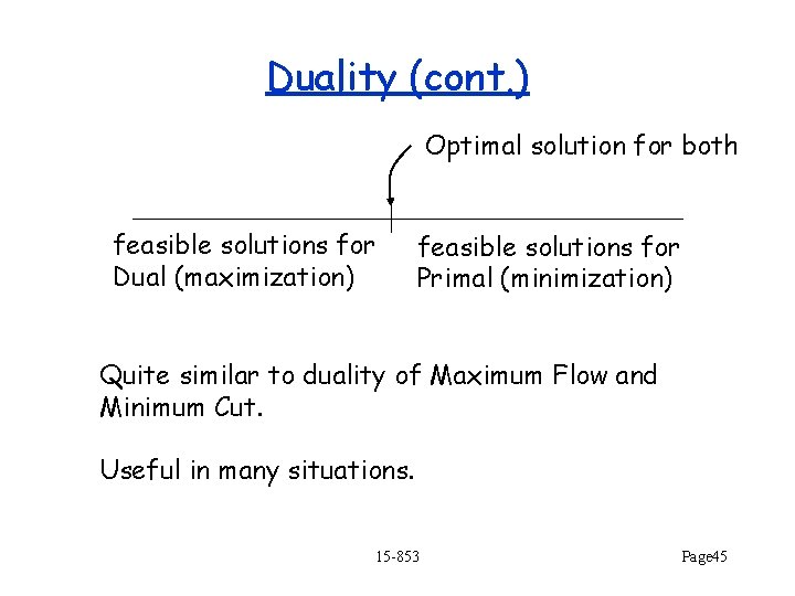
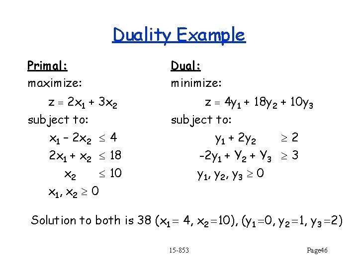
Duality Primal (P): maximize z c. Tx subject to Ax b x 0 (n equations, m variables) Dual (D): minimize z y. Tb subject to ATy c y 0 (m equations, n variables) Duality Theorem: if x is feasible for P and y is feasible for D, then cx yb and at optimality cx yb. 15 -853 Page 44

Duality (cont. ) Optimal solution for both feasible solutions for Dual (maximization) feasible solutions for Primal (minimization) Quite similar to duality of Maximum Flow and Minimum Cut. Useful in many situations. 15 -853 Page 45

Duality Example Primal: maximize: Dual: minimize: z 2 x 1 + 3 x 2 subject to: x 1 – 2 x 2 4 2 x 1 + x 2 18 10 x 2 x 1, x 2 0 z 4 y 1 + 18 y 2 + 10 y 3 subject to: 2 y 1 + 2 y 2 -2 y 1 + Y 2 + Y 3 3 y 1, y 2 , y 3 0 Solution to both is 38 (x 1 4, x 2 10), (y 1 0, y 2 1, y 3 2) 15 -853 Page 46

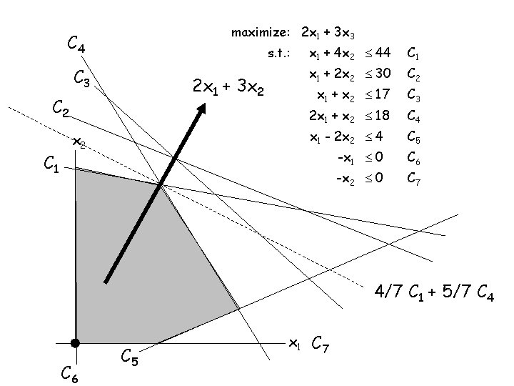
maximize: 2 x 1 + 3 x 3 C 4 s. t. : C 3 2 x 1 + 3 x 2 C 1 x 2 x 1 + 4 x 2 44 C 1 x 1 + 2 x 2 30 C 2 x 1 + x 2 17 C 3 2 x 1 + x 2 18 C 4 x 1 - 2 x 2 4 C 5 -x 1 0 C 6 -x 2 0 C 7 4/7 C 1 + 5/7 C 4 C 6 C 5 x 1 C 7