14 pierep1 12 pierep1 24 col rainbow24 pierep1

) pie(rep(1, 24), col = rainbow(24)) pie(rep(1, 24), col")
파이 차트 컬러 1/4 pie(rep(1, 12)) pie(rep(1, 24), col = rainbow(24)) pie(rep(1, 24), col = heat. colors(24)) 7
, col = terrain. colors(24)) pie(rep(1, 24), col =")
파이 차트 컬러 2/4 pie(rep(1, 24), col = terrain. colors(24)) pie(rep(1, 24), col = topo. colors(24)) pie(rep(1, 24), col = cm. colors(24)) 8

파이 차트 컬러 3/4 pie. sales <- c(0. 12, 0. 3, 0. 26, 0. 16, 0. 04, 0. 12) names(pie. sales) <- c("Blueberry", "Cherry", "Apple", "Boston Cream", "Other", "Vanilla Cream") pie(pie. sales, col = c("purple", "violetred 1", "green 3", "cornsilk", "cyan", "white")) 9

파이 차트 컬러 4/4 ## (original by Final. Backwards. Glance ## on http: //imgur. com/gallery/w. Wrp. U 4 X) pie(c(Sky = 78, "Sunny side of pyramid" = 17, "Shady side of pyramid" = 5), init. angle = 315, col = c("deepskyblue", "yellow 3"), border = FALSE) 10

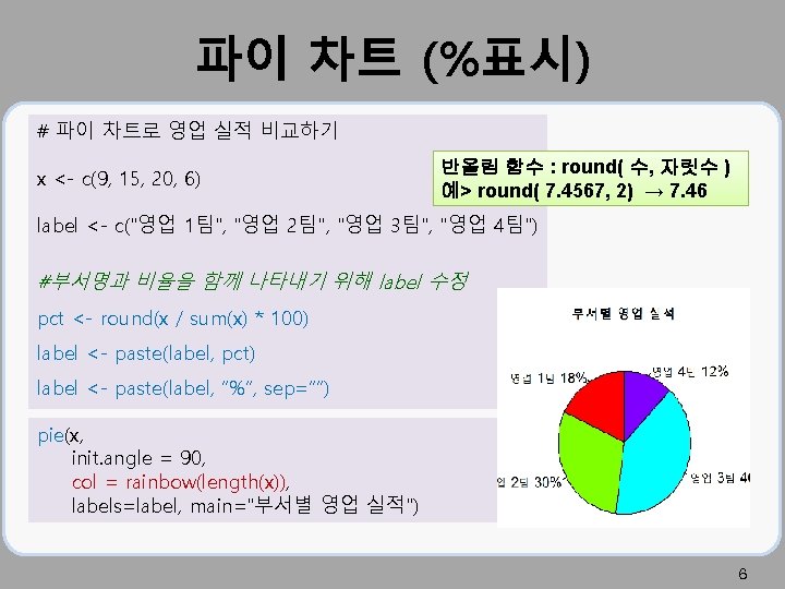
3차원 파이 차트 # 파이 차트로 영업 실적 비교하기 x <- c(9, 15, 20, 6) pct <- round(x / sum(x) * 100) label <- c("영업 1팀", "영업 2팀", "영업 3팀", "영업 4팀") label <- paste(label, pct) label <- paste(label, “%”, sep=“”) install. packages("plotrix") #3차원 pie 3 D 함수사용 library(plotrix) pie 3 D(x, labels=label, explode=0. 1, labelcex=0. 8, main="부서별 영업 실적") 부채꼴 간격 라벨문자크기 * 0. 8 11
 name <- c(\"영업 1팀\", \"영업")
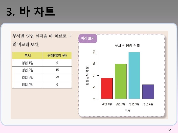
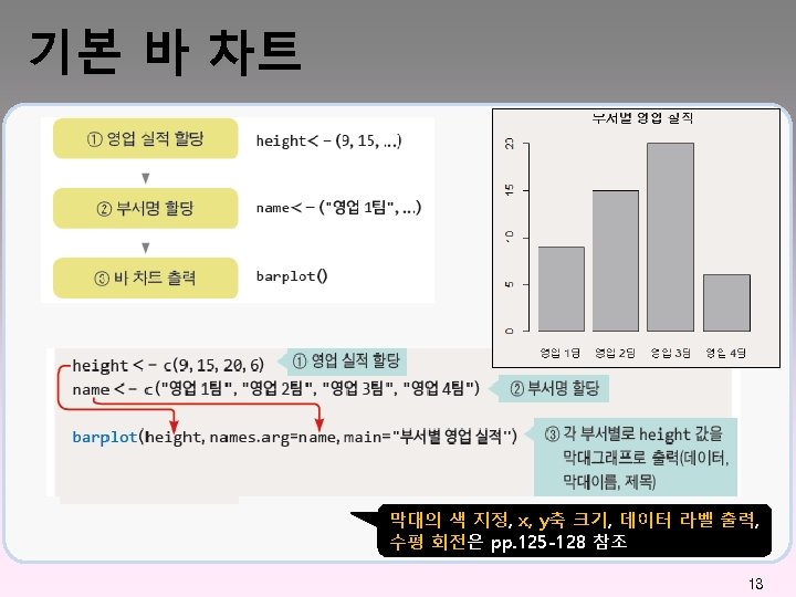
바 차트 컬러 height <- c(9, 15, 20, 6) name <- c("영업 1팀", "영업 2팀", "영업 3팀", "영업 4팀") barplot(height, names. arg=name, main="부서별 영업 실적“, col=rainbow(length(height))) 14
\") barplot(height,")
바 차트 라벨 barplot(height, names. arg=name, main="부서별 영업 실적“, xlab="부서", ylab="영업 실적(억 원)") barplot(height, names. arg=name, main="부서별 영업 실적", col=rainbow(length(height)), xlab="부서", ylab="영업 실적(억 원)", ylim=c(0, 25)) 15

바 차트 데이터 라벨 위치 bp <- barplot(height, names. arg=name, main="부서별 영업 실적“, xlab="부서", ylab="영업 실적(억 원)") text(x=bp, y=height, labels=round(height, 0), pos=3) text(x=bp, y=height, labels=round(height, 0), pos=1) pos=1 pos=2 pos=3 pos=4 아래쪽 왼쪽 위쪽 오른쪽 16
), xlab=\"영업 실적(억 원)\", ylab=\"부서\",")
바 차트 회전하기 barplot(height, names. arg=name, main="부서별 영업 실적", col=rainbow(length(height)), xlab="영업 실적(억 원)", ylab="부서", horiz=TRUE, width=50) # 50 pixel width 18
 barplot(height, main=\"부서별 영업 실적\", names.")
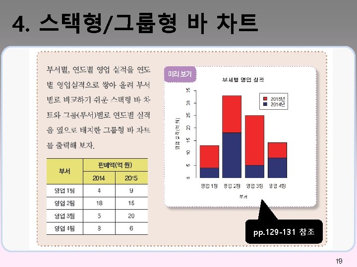
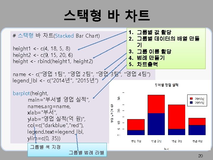
그룹형 바 차트 # 그룹형 바 차트(Grouped Bar Chart) barplot(height, main="부서별 영업 실적", names. arg=name, xlab="부서", ylab="영업 실적(억 원)", col=c("darkblue", "red"), legend. text=legend_lbl, ylim=c(0, 30), beside=TRUE, #막대 옆으로 배치 args. legend=list(x='top')) #범례 위중앙에 배치 21
 women height 1 58 2 59 3 60")
R 내장 women 데이터 세트 data(women) women height 1 58 2 59 3 60 4 61 5 62. . . 12 69 13 70 14 71 15 72 # obsolete convention # just use women weight 115 117 120 123 126 150 154 159 164 23
 height <- women$height plot(height, weight, xlab=\"키\", ylab=\"몸무게\")")
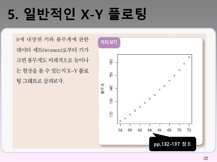
일반적인 X-Y 플로팅 weight <- women$weight plot(weight) height <- women$height plot(height, weight, xlab="키", ylab="몸무게") 24
의 type 1/4 plot(height, weight, xlab=\"키\", ylab=\"몸무게\", type=\"p\") plot(height, weight, xlab=\"키\", ylab=\"몸무게\", type=\"l\") 25")
plot()의 type 1/4 plot(height, weight, xlab="키", ylab="몸무게", type="p") plot(height, weight, xlab="키", ylab="몸무게", type="l") 25
의 type 2/4 plot(height, plot(height, plot(height, weight, weight, weight, xlab=\"키\", xlab=\"키\", xlab=\"키\", ylab=\"몸무게\", ylab=\"몸무게\",")
plot()의 type 2/4 plot(height, plot(height, plot(height, weight, weight, weight, xlab="키", xlab="키", xlab="키", ylab="몸무게", ylab="몸무게", ylab="몸무게", "p" "l" "b" "c" "o" "h" "s" "S" "n" type="p") type="l") type="b") type="c") type="o") type="h") type="s") type="S") type="n") for for for points lines both the lines part alone of "b" both 'overplotted' 'histogram' like vertical lines stair steps other steps no plotting 26
 'type' Example 3/4 x <- c(1: 5) y <- c(1: 5) par(pch=22, col=\"red\")")
plot() 'type' Example 3/4 x <- c(1: 5) y <- c(1: 5) par(pch=22, col="red") par(mfrow=c(2, 4)) opts = c("p", "l", "b", "c", "o", "s", "S", "h") for( i in 1: length(opts) ) { heading = paste("type =", opts[i]) plot(x, y, type="n", main=heading) lines(x, y, type=opts[i]) } 27
의 type 3/3 28")
plot()의 type 3/3 28

X-Y 플로팅 문자의 변경 weight <- women$weight height <- women$height plot(height, weight, xlab="키", ylab="몸무게", pch=23, col="blue", bg="yellow", cex=1. 5) 29

 hist(mag, main=\"지진 발생")
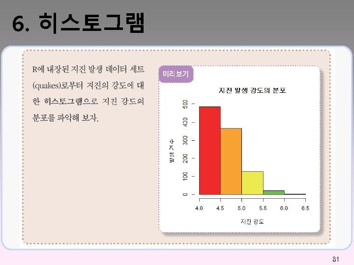
히스토그램 컬러 colors <- c("red", "orange", "yellow", "green", "blue", "navy", "violet") hist(mag, main="지진 발생 강도의 분포", xlab="지진 강도", ylab="발생 건수", col=colors, breaks=seq(4, 6. 5, by=0. 5)) 34

히스토그램 빈도수 hist(mag, main="지진 발생 강도의 분포", xlab="지진 강도", ylab="상대도수", col=colors, breaks=seq(4, 6. 5, by=0. 5), freq=FALSE) 35
 37")
히스토그램 breaks hist(mag, main="지진 발생 강도의 분포", xlab="지진 강도", ylab="상대도수", col=colors, breaks="Sturges", freq=FALSE) 37
 박스 플롯 관련 통계 데이터 살펴보기 mag <- quakes$mag head(mag)")
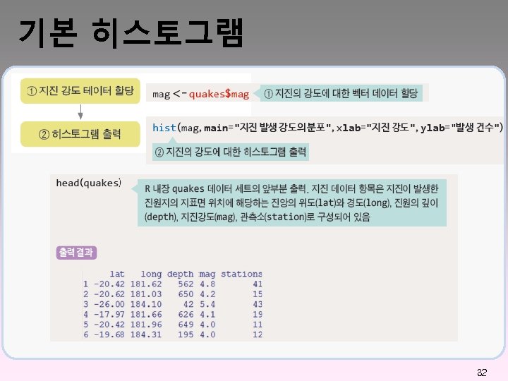
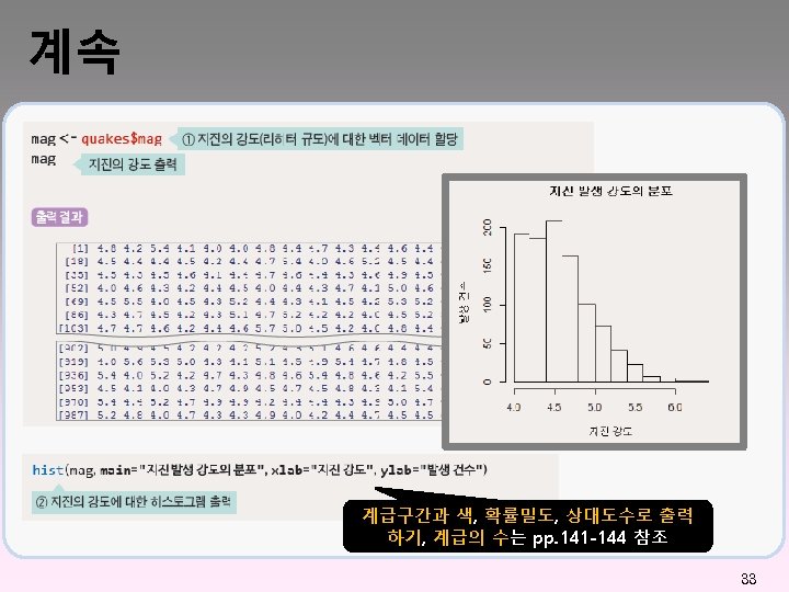
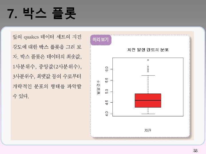
박스 플롯 (Box Plot) 박스 플롯 관련 통계 데이터 살펴보기 mag <- quakes$mag head(mag) [1] 4. 8 4. 2 5. 4 4. 1 4. 0 min(mag) [1] 4 max(mag) [1] 6. 4 median(mag) [1] 4. 6 quantile(mag, c(0. 25, 0. 75)) 25% 50% 75% 4. 3 4. 6 4. 9 39
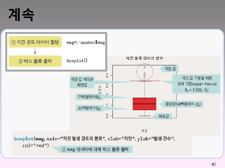
- Slides: 40