14 PARTIAL DERIVATIVES PARTIAL DERIVATIVES So far we

14 PARTIAL DERIVATIVES

PARTIAL DERIVATIVES So far, we have dealt with the calculus of functions of a single variable. However, in the real world, physical quantities often depend on two or more variables.

PARTIAL DERIVATIVES So, in this chapter, we: § Turn our attention to functions of several variables. § Extend the basic ideas of differential calculus to such functions.

PARTIAL DERIVATIVES 14. 1 Functions of Several Variables In this section, we will learn about: Functions of two or more variables and how to produce their graphs.

FUNCTIONS OF SEVERAL VARIABLES In this section, we study functions of two or more variables from four points of view: § Verbally (a description in words) § Numerically (a table of values) § Algebraically (an explicit formula) § Visually (a graph or level curves)

FUNCTIONS OF TWO VARIABLES The temperature T at a point on the surface of the earth at any given time depends on the longitude x and latitude y of the point. § We can think of T as being a function of the two variables x and y, or as a function of the pair (x, y). § We indicate this functional dependence by writing: T = f(x, y)

FUNCTIONS OF TWO VARIABLES The volume V of a circular cylinder depends on its radius r and its height h. § In fact, we know that V = πr 2 h. § We say that V is a function of r and h. § We write V(r, h) = πr 2 h.

FUNCTION OF TWO VARIABLES A function f of two variables is a rule that assigns to each ordered pair of real numbers (x, y) in a set D a unique real number denoted by (x, y). § The set D is the domain of f. § Its range is the set of values that f takes on, that is, {f(x, y) | (x, y) D}

FUNCTIONS OF TWO VARIABLES We often write z = f(x, y) to make explicit the value taken on by f at the general point (x, y). § The variables x and y are independent variables. § z is the dependent variable. § Compare this with the notation y = f(x) for functions of a single variable.

FUNCTIONS OF TWO VARIABLES A function of two variables is just a function whose: § Domain is a subset of R 2 § Range is a subset of R

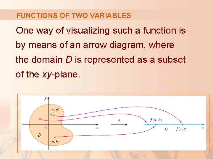
FUNCTIONS OF TWO VARIABLES One way of visualizing such a function is by means of an arrow diagram, where the domain D is represented as a subset of the xy-plane.

FUNCTIONS OF TWO VARIABLES If a function f is given by a formula and no domain is specified, then the domain of f is understood to be: § The set of all pairs (x, y) for which the given expression is a well-defined real number.

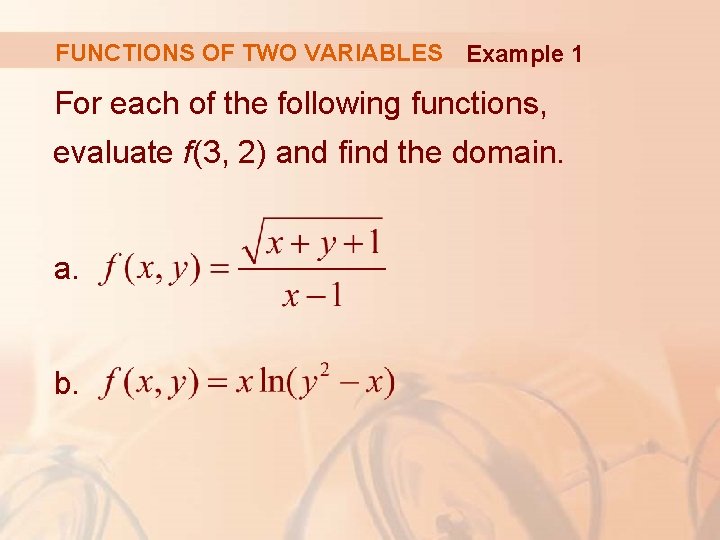
FUNCTIONS OF TWO VARIABLES Example 1 For each of the following functions, evaluate f(3, 2) and find the domain. a. b.

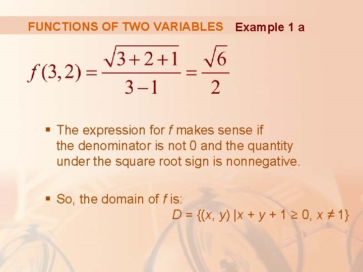
FUNCTIONS OF TWO VARIABLES Example 1 a § The expression for f makes sense if the denominator is not 0 and the quantity under the square root sign is nonnegative. § So, the domain of f is: D = {(x, y) |x + y + 1 ≥ 0, x ≠ 1}

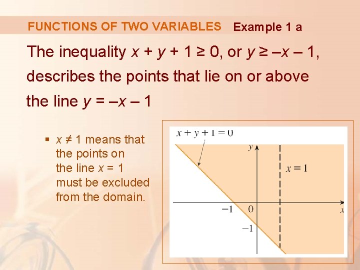
FUNCTIONS OF TWO VARIABLES Example 1 a The inequality x + y + 1 ≥ 0, or y ≥ –x – 1, describes the points that lie on or above the line y = –x – 1 § x ≠ 1 means that the points on the line x = 1 must be excluded from the domain.

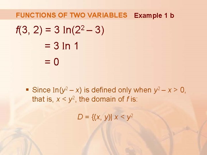
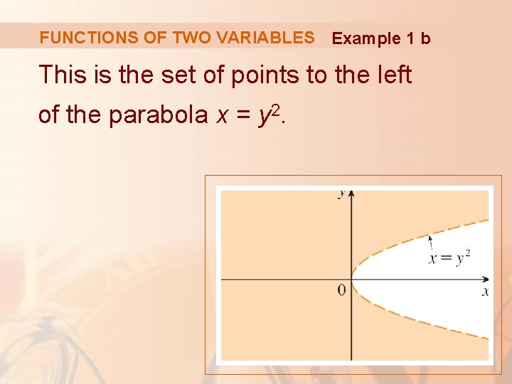
FUNCTIONS OF TWO VARIABLES Example 1 b f(3, 2) = 3 ln(22 – 3) = 3 ln 1 =0 § Since ln(y 2 – x) is defined only when y 2 – x > 0, that is, x < y 2, the domain of f is: D = {(x, y)| x < y 2

FUNCTIONS OF TWO VARIABLES Example 1 b This is the set of points to the left of the parabola x = y 2.

FUNCTIONS OF TWO VARIABLES Not all functions are given by explicit formulas. § The function in the next example is described verbally and by numerical estimates of its values.

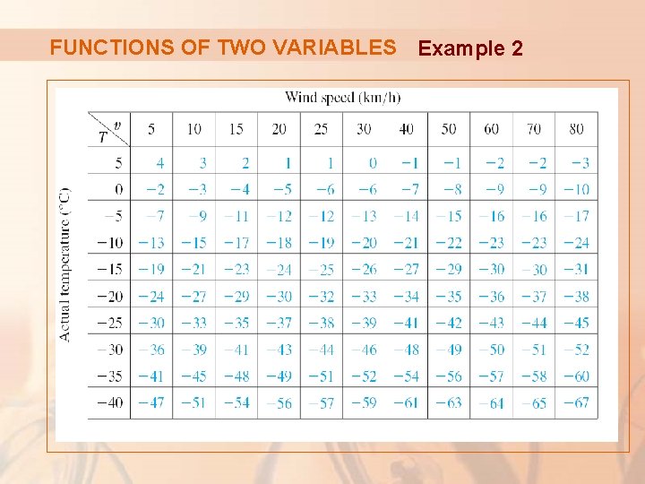
FUNCTIONS OF TWO VARIABLES Example 2 In regions with severe winter weather, the wind-chill index is often used to describe the apparent severity of the cold. § This index W is a subjective temperature that depends on the actual temperature T and the wind speed v. § So, W is a function of T and v, and we can write: W = f(T, v)

FUNCTIONS OF TWO VARIABLES Example 2 The following table records values of W compiled by the NOAA National Weather Service of the US and the Meteorological Service of Canada.

FUNCTIONS OF TWO VARIABLES Example 2

FUNCTIONS OF TWO VARIABLES Example 2 For instance, the table shows that, if the temperature is – 5°C and the wind speed is 50 km/h, then subjectively it would feel as cold as a temperature of about – 15°C with no wind. § Therefore, f(– 5, 50) = – 15

FUNCTIONS OF TWO VARIABLES Example 3 In 1928, Charles Cobb and Paul Douglas published a study in which they modeled the growth of the American economy during the period 1899– 1922.

FUNCTIONS OF TWO VARIABLES Example 3 They considered a simplified view in which production output is determined by the amount of labor involved and the amount of capital invested. § While there are many other factors affecting economic performance, their model proved to be remarkably accurate.

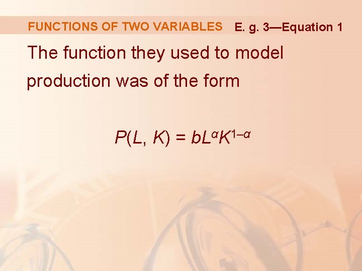
FUNCTIONS OF TWO VARIABLES E. g. 3—Equation 1 The function they used to model production was of the form P(L, K) = b. LαK 1–α

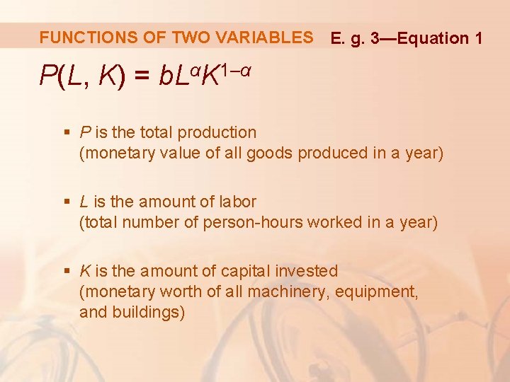
FUNCTIONS OF TWO VARIABLES E. g. 3—Equation 1 P(L, K) = b. LαK 1–α § P is the total production (monetary value of all goods produced in a year) § L is the amount of labor (total number of person-hours worked in a year) § K is the amount of capital invested (monetary worth of all machinery, equipment, and buildings)

FUNCTIONS OF TWO VARIABLES Example 3 In Section 14. 3, we will show the form of Equation 1 follows from certain economic assumptions.

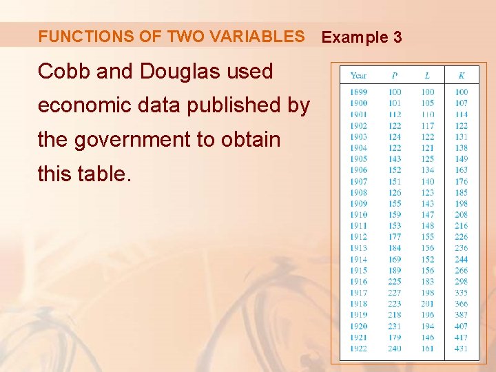
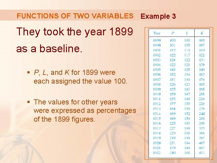
FUNCTIONS OF TWO VARIABLES Example 3 Cobb and Douglas used economic data published by the government to obtain this table.

FUNCTIONS OF TWO VARIABLES Example 3 They took the year 1899 as a baseline. § P, L, and K for 1899 were each assigned the value 100. § The values for other years were expressed as percentages of the 1899 figures.

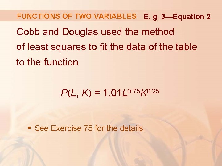
FUNCTIONS OF TWO VARIABLES E. g. 3—Equation 2 Cobb and Douglas used the method of least squares to fit the data of the table to the function P(L, K) = 1. 01 L 0. 75 K 0. 25 § See Exercise 75 for the details.

FUNCTIONS OF TWO VARIABLES Example 3 Let’s use the model given by the function in Equation 2 to compute the production in the years 1910 and 1920.

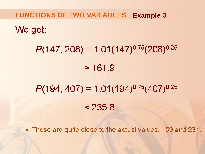
FUNCTIONS OF TWO VARIABLES Example 3 We get: P(147, 208) = 1. 01(147)0. 75(208)0. 25 ≈ 161. 9 P(194, 407) = 1. 01(194)0. 75(407)0. 25 ≈ 235. 8 § These are quite close to the actual values, 159 and 231.

COBB-DOUGLAS PRODN. FUNCN. Example 3 The production function (Equation 1) has subsequently been used in many settings, ranging from individual firms to global economic questions. § It has become known as the Cobb-Douglas production function.

COBB-DOUGLAS PRODN. FUNCN. Example 3 Its domain is: {(L, K) | L ≥ 0, K ≥ 0} § This is because L and K represent labor and capital and so are never negative.

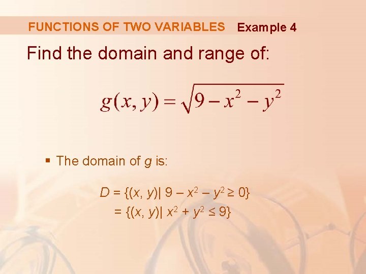
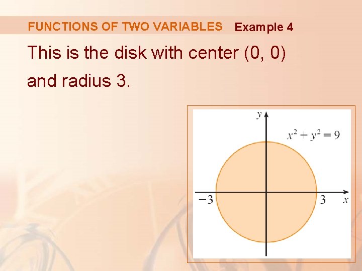
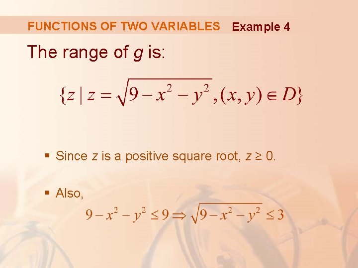
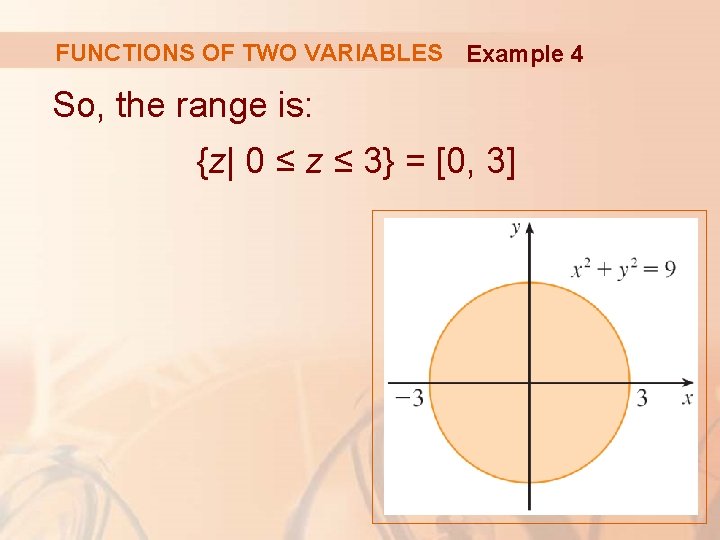
FUNCTIONS OF TWO VARIABLES Example 4 Find the domain and range of: § The domain of g is: D = {(x, y)| 9 – x 2 – y 2 ≥ 0} = {(x, y)| x 2 + y 2 ≤ 9}

FUNCTIONS OF TWO VARIABLES Example 4 This is the disk with center (0, 0) and radius 3.

FUNCTIONS OF TWO VARIABLES Example 4 The range of g is: § Since z is a positive square root, z ≥ 0. § Also,

FUNCTIONS OF TWO VARIABLES Example 4 So, the range is: {z| 0 ≤ z ≤ 3} = [0, 3]

GRAPHS Another way of visualizing the behavior of a function of two variables is to consider its graph.

GRAPH If f is a function of two variables with domain D, then the graph of f is the set of all points (x, y, z) in R 3 such that z = f(x, y) and (x, y) is in D.

GRAPHS Just as the graph of a function f of one variable is a curve C with equation y = f(x), so the graph of a function f of two variables is: § A surface S with equation z = f(x, y)

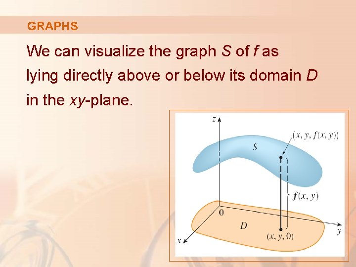
GRAPHS We can visualize the graph S of f as lying directly above or below its domain D in the xy-plane.

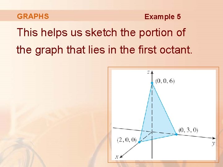
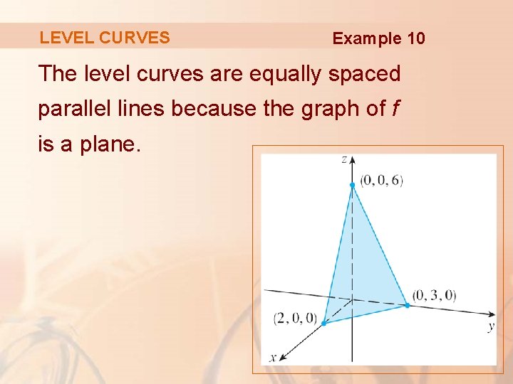
GRAPHS Example 5 Sketch the graph of the function f(x, y) = 6 – 3 x – 2 y § The graph of f has the equation z = 6 – 3 x – 2 y or 3 x + 2 y + z = 6 § This represents a plane.

GRAPHS Example 5 To graph the plane, we first find the intercepts. § Putting y = z = 0 in the equation, we get x = 2 as the x-intercept. § Similarly, the y-intercept is 3 and the z-intercept is 6.

GRAPHS Example 5 This helps us sketch the portion of the graph that lies in the first octant.

LINEAR FUNCTION The function in Example 5 is a special case of the function f(x, y) = ax + by + c § It is called a linear function.

LINEAR FUNCTIONS The graph of such a function has the equation z = ax + by + c or ax + by – z + c = 0 § Thus, it is a plane.

LINEAR FUNCTIONS In much the same way that linear functions of one variable are important in single-variable calculus, we will see that: § Linear functions of two variables play a central role in multivariable calculus.

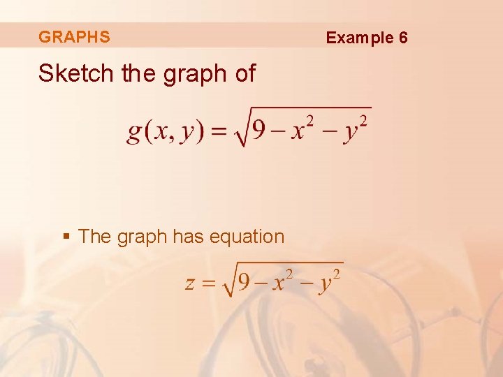
GRAPHS Sketch the graph of § The graph has equation Example 6

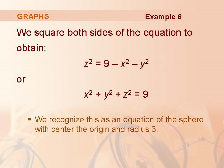
GRAPHS Example 6 We square both sides of the equation to obtain: z 2 = 9 – x 2 – y 2 or x 2 + y 2 + z 2 = 9 § We recognize this as an equation of the sphere with center the origin and radius 3.

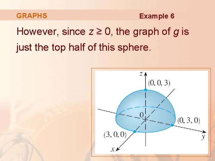
GRAPHS Example 6 However, since z ≥ 0, the graph of g is just the top half of this sphere.

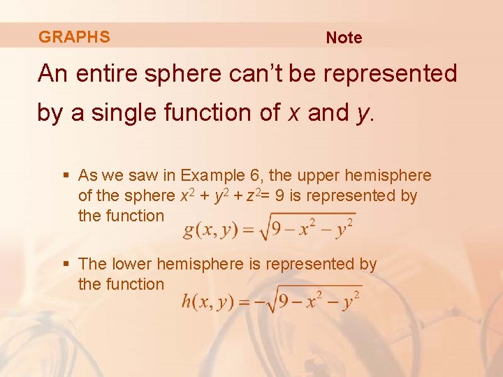
GRAPHS Note An entire sphere can’t be represented by a single function of x and y. § As we saw in Example 6, the upper hemisphere of the sphere x 2 + y 2 + z 2= 9 is represented by the function § The lower hemisphere is represented by the function

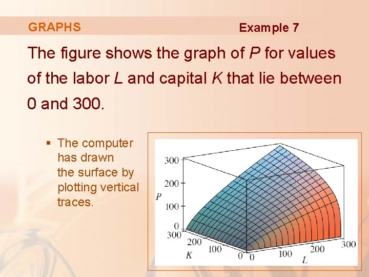
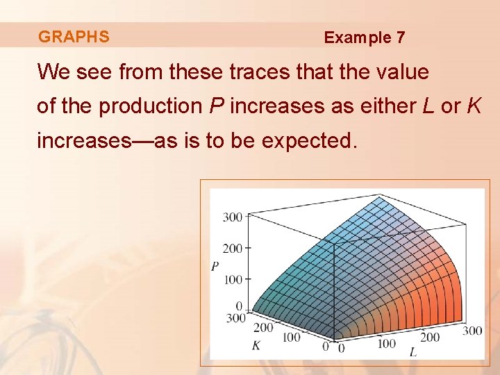
GRAPHS Example 7 Use a computer to draw the graph of the Cobb-Douglas production function P(L, K) = 1. 01 L 0. 75 K 0. 25

GRAPHS Example 7 The figure shows the graph of P for values of the labor L and capital K that lie between 0 and 300. § The computer has drawn the surface by plotting vertical traces.

GRAPHS Example 7 We see from these traces that the value of the production P increases as either L or K increases—as is to be expected.

GRAPHS Example 8 Find the domain and range and sketch the graph of h(x, y) = 4 x 2 + y 2

GRAPHS Example 8 Notice that h(x, y) is defined for all possible ordered pairs of real numbers (x, y). § So, the domain is R 2, the entire xy-plane.

GRAPHS Example 8 The range of h is the set [0, ∞) of all nonnegative real numbers. § Notice that x 2 ≥ 0 and y 2 ≥ 0. § So, h(x, y) ≥ 0 for all x and y.

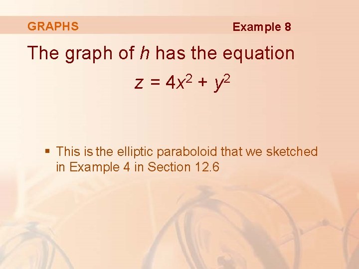
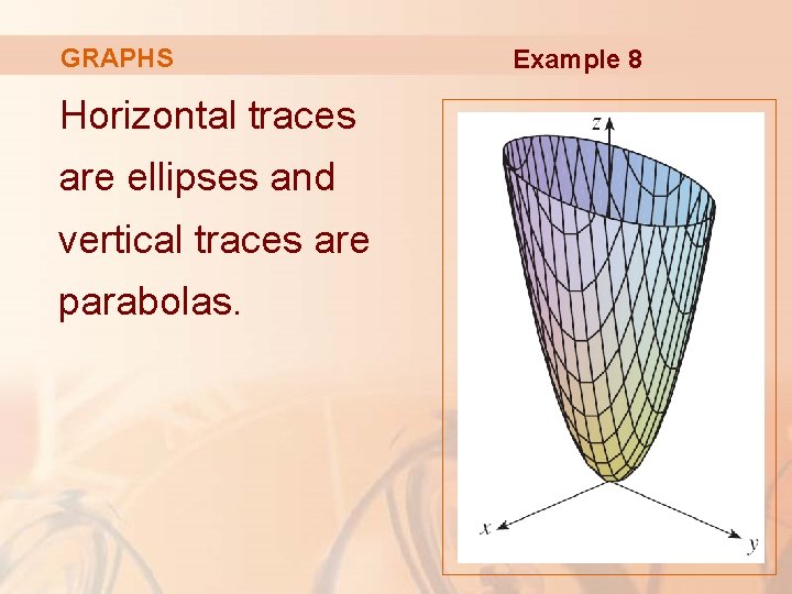
GRAPHS Example 8 The graph of h has the equation z = 4 x 2 + y 2 § This is the elliptic paraboloid that we sketched in Example 4 in Section 12. 6

GRAPHS Horizontal traces are ellipses and vertical traces are parabolas. Example 8

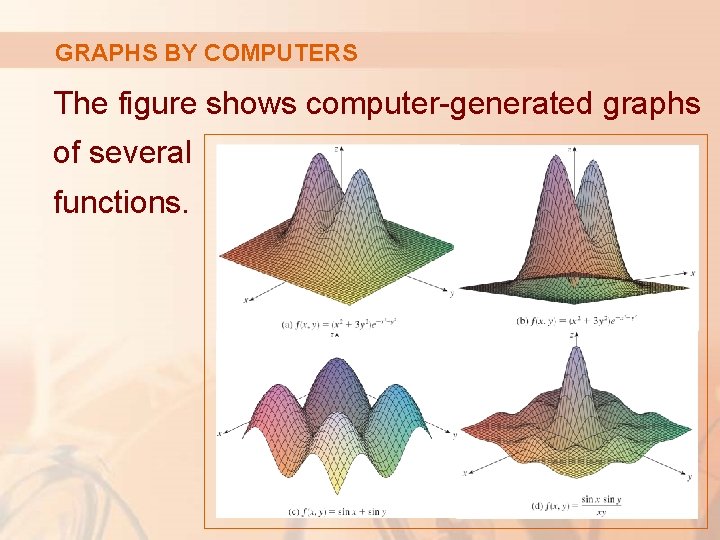
GRAPHS BY COMPUTERS Computer programs are readily available for graphing functions of two variables. In most such programs, § Traces in the vertical planes x = k and y = k are drawn for equally spaced values of k. § Parts of the graph are eliminated using hidden line removal.

GRAPHS BY COMPUTERS The figure shows computer-generated graphs of several functions.

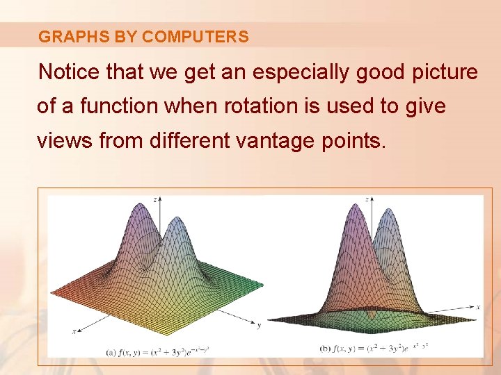
GRAPHS BY COMPUTERS Notice that we get an especially good picture of a function when rotation is used to give views from different vantage points.

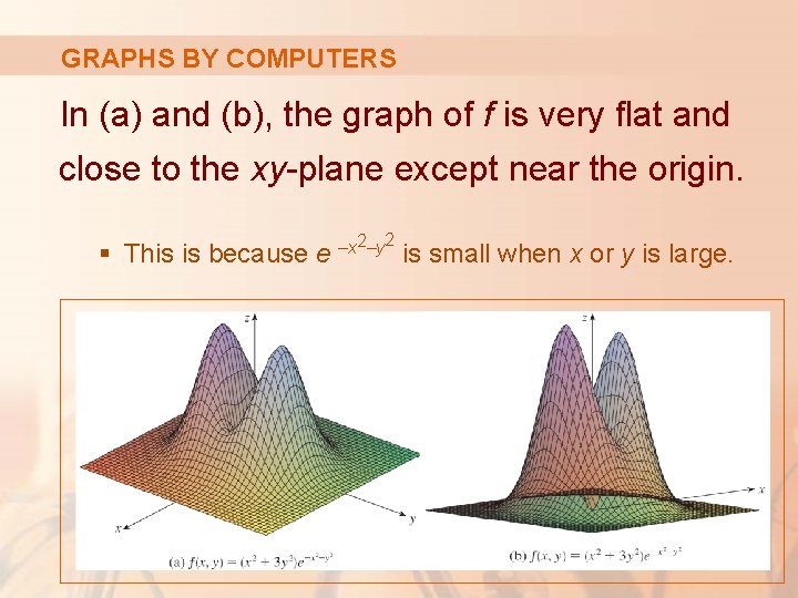
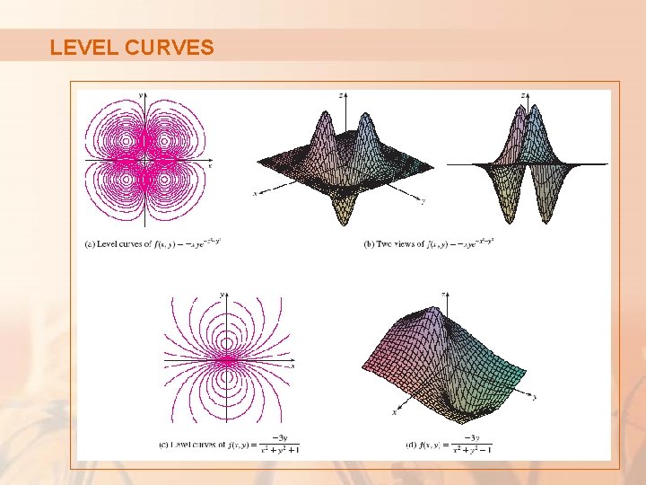
GRAPHS BY COMPUTERS In (a) and (b), the graph of f is very flat and close to the xy-plane except near the origin. § This is because e –x 2–y 2 is small when x or y is large.

LEVEL CURVES So far, we have two methods for visualizing functions, arrow diagrams and graphs. § A third method, borrowed from mapmakers, is a contour map on which points of constant elevation are joined to form contour curves, or level curves.

LEVEL CURVES Definition The level curves of a function f of two variables are the curves with equations f(x, y) = k where k is a constant (in the range of f).

LEVEL CURVE A level curve f(x, y) = k is the set of all points in the domain of f at which f takes on a given value k. § That is, it shows where the graph of f has height k.

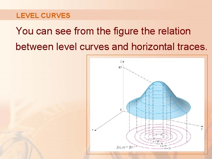
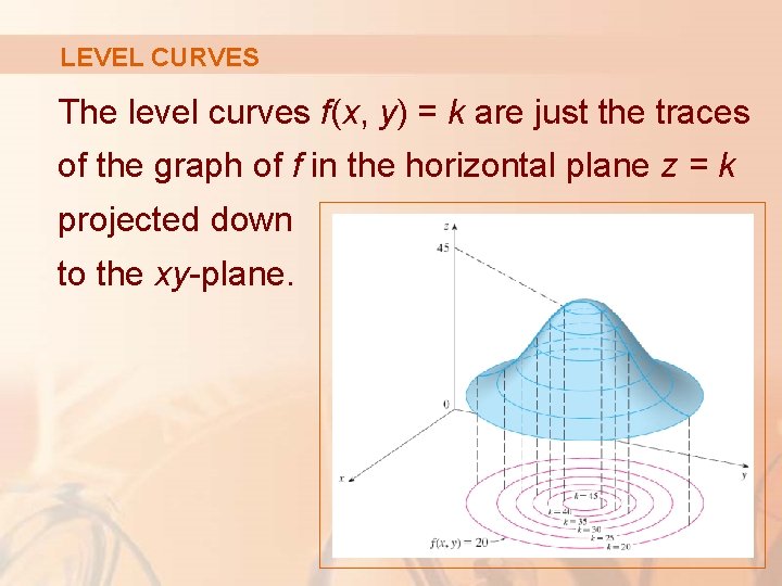
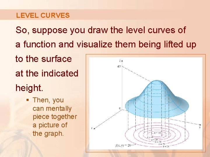
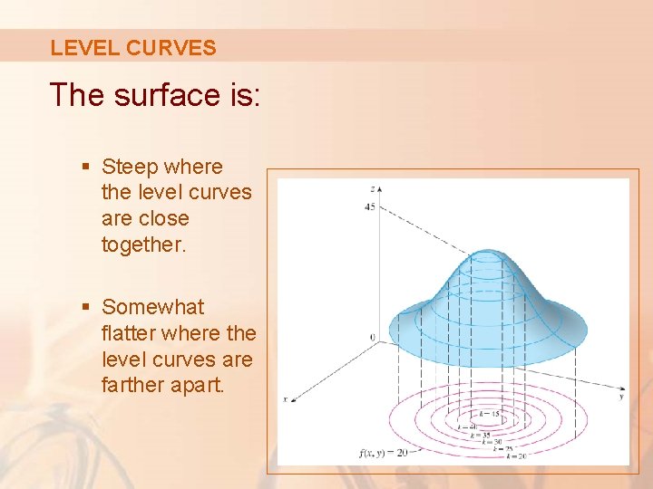
LEVEL CURVES You can see from the figure the relation between level curves and horizontal traces.

LEVEL CURVES The level curves f(x, y) = k are just the traces of the graph of f in the horizontal plane z = k projected down to the xy-plane.

LEVEL CURVES So, suppose you draw the level curves of a function and visualize them being lifted up to the surface at the indicated height. § Then, you can mentally piece together a picture of the graph.

LEVEL CURVES The surface is: § Steep where the level curves are close together. § Somewhat flatter where the level curves are farther apart.

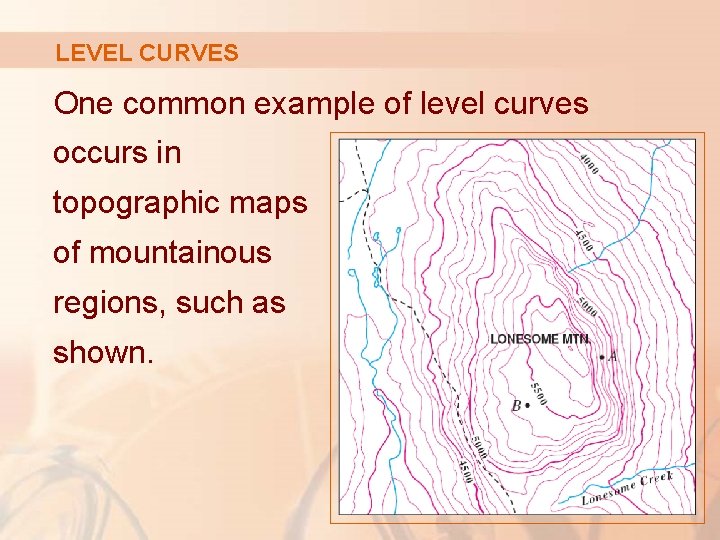
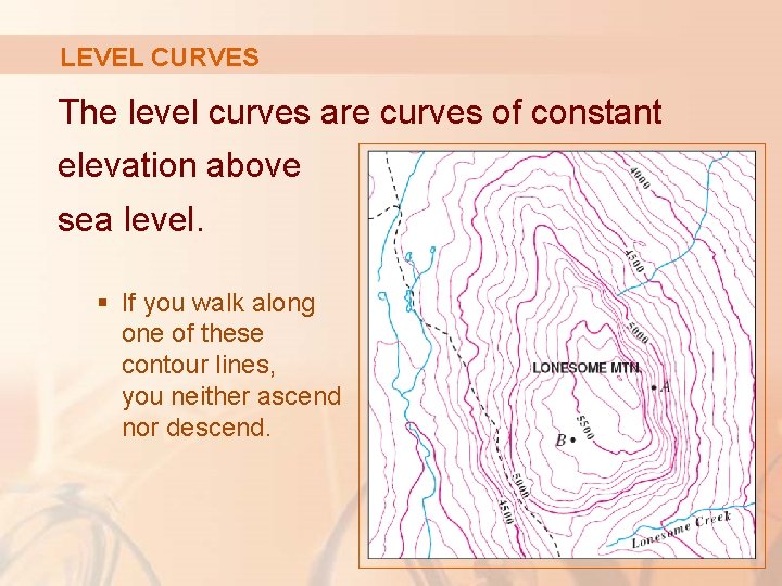
LEVEL CURVES One common example of level curves occurs in topographic maps of mountainous regions, such as shown.

LEVEL CURVES The level curves are curves of constant elevation above sea level. § If you walk along one of these contour lines, you neither ascend nor descend.

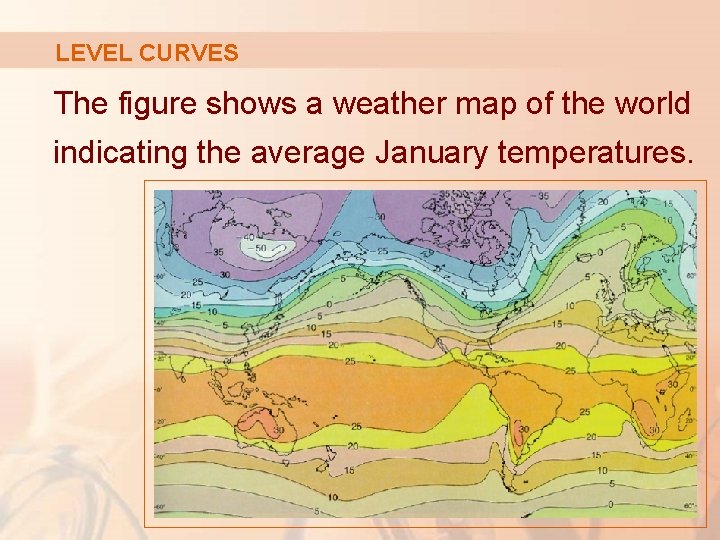
LEVEL CURVES Another common example is the temperature function introduced in the opening paragraph of the section. § Here, the level curves are called isothermals. § They join locations with the same temperature.

LEVEL CURVES The figure shows a weather map of the world indicating the average January temperatures.

LEVEL CURVES The isothermals are the curves that separate the colored bands.

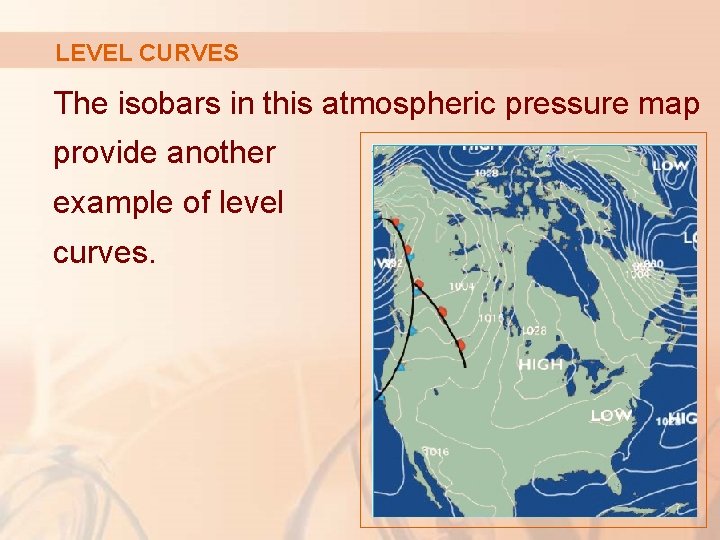
LEVEL CURVES The isobars in this atmospheric pressure map provide another example of level curves.

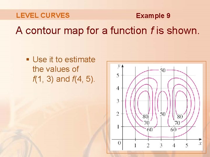
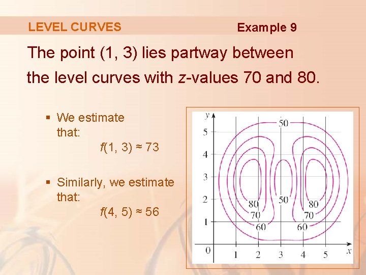
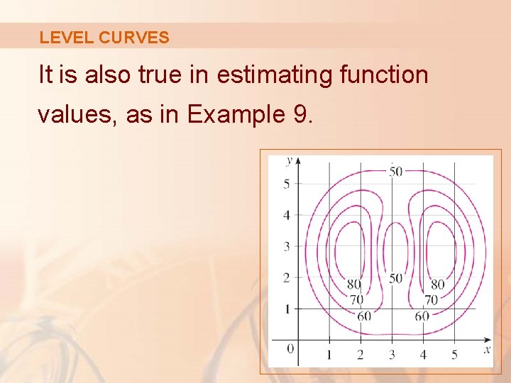
LEVEL CURVES Example 9 A contour map for a function f is shown. § Use it to estimate the values of f(1, 3) and f(4, 5).

LEVEL CURVES Example 9 The point (1, 3) lies partway between the level curves with z-values 70 and 80. § We estimate that: f(1, 3) ≈ 73 § Similarly, we estimate that: f(4, 5) ≈ 56

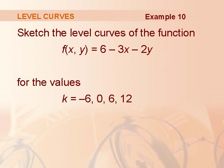
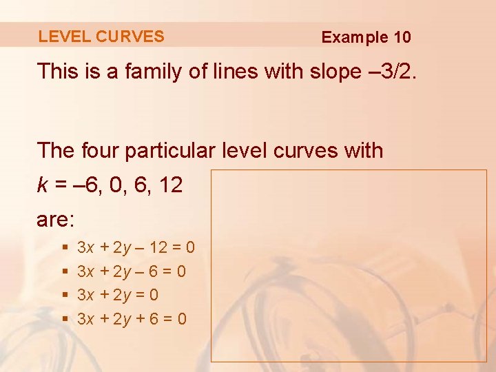
LEVEL CURVES Example 10 Sketch the level curves of the function f(x, y) = 6 – 3 x – 2 y for the values k = – 6, 0, 6, 12

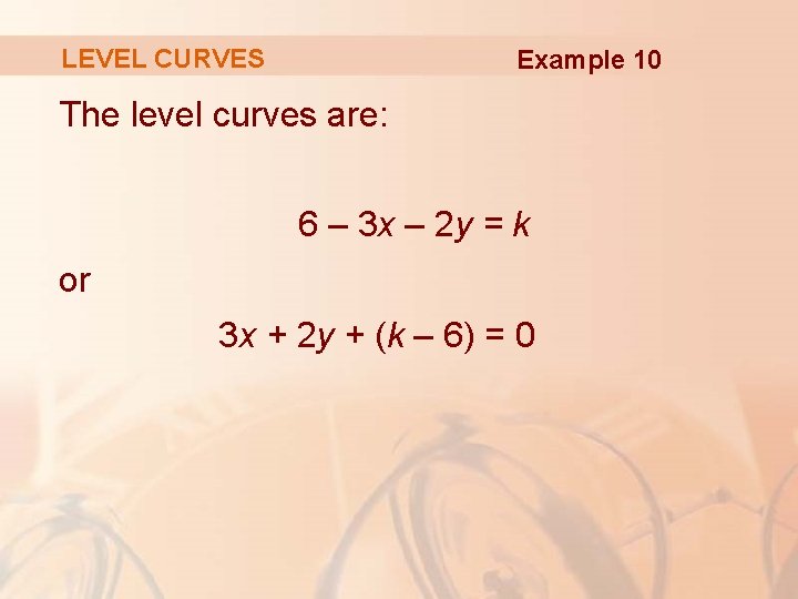
LEVEL CURVES Example 10 The level curves are: 6 – 3 x – 2 y = k or 3 x + 2 y + (k – 6) = 0

LEVEL CURVES Example 10 This is a family of lines with slope – 3/2. The four particular level curves with k = – 6, 0, 6, 12 are: § § 3 x + 2 y – 12 = 0 3 x + 2 y – 6 = 0 3 x + 2 y + 6 = 0

LEVEL CURVES Example 10 The level curves are equally spaced parallel lines because the graph of f is a plane.

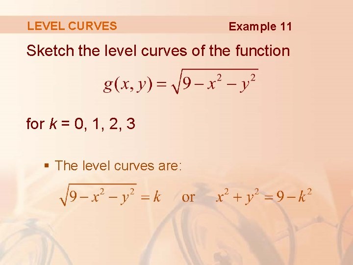
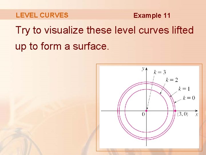
LEVEL CURVES Example 11 Sketch the level curves of the function for k = 0, 1, 2, 3 § The level curves are:

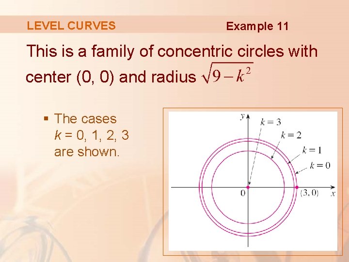
LEVEL CURVES Example 11 This is a family of concentric circles with center (0, 0) and radius § The cases k = 0, 1, 2, 3 are shown.

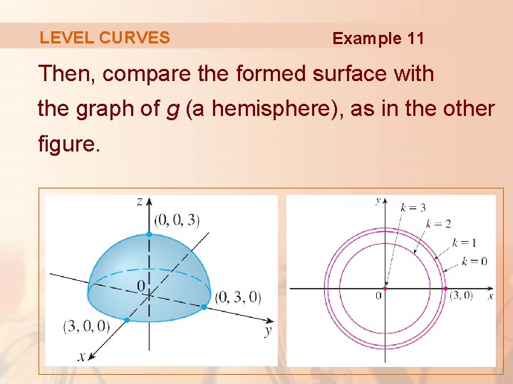
LEVEL CURVES Example 11 Try to visualize these level curves lifted up to form a surface.

LEVEL CURVES Example 11 Then, compare the formed surface with the graph of g (a hemisphere), as in the other figure.

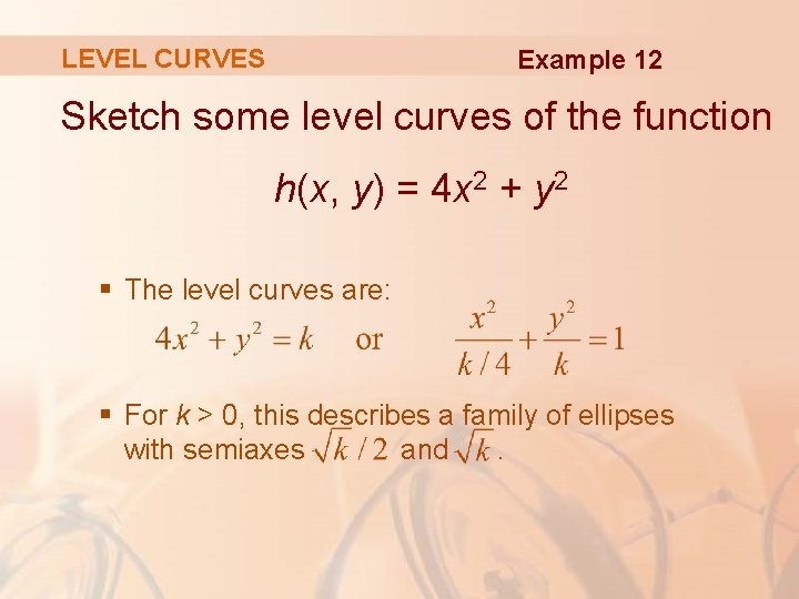
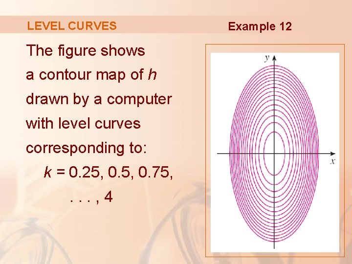
LEVEL CURVES Example 12 Sketch some level curves of the function h(x, y) = 4 x 2 + y 2 § The level curves are: § For k > 0, this describes a family of ellipses with semiaxes and.

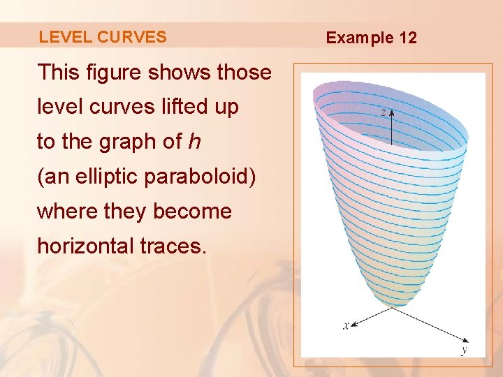
LEVEL CURVES The figure shows a contour map of h drawn by a computer with level curves corresponding to: k = 0. 25, 0. 75, . . . , 4 Example 12

LEVEL CURVES This figure shows those level curves lifted up to the graph of h (an elliptic paraboloid) where they become horizontal traces. Example 12

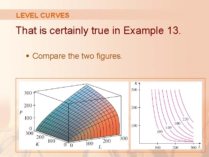
LEVEL CURVES Example 13 Plot level curves for the Cobb-Douglas production function of Example 3.

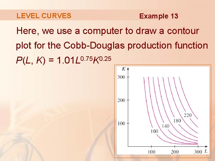
LEVEL CURVES Example 13 Here, we use a computer to draw a contour plot for the Cobb-Douglas production function P(L, K) = 1. 01 L 0. 75 K 0. 25

LEVEL CURVES Example 13 Level curves are labeled with the value of the production P. § For instance, the level curve labeled 140 shows all values of the labor L and capital investment K that result in a production of P = 140.

LEVEL CURVES Example 13 We see that, for a fixed value of P, as L increases K decreases, and vice versa.

LEVEL CURVES For some purposes, a contour map is more useful than a graph.

LEVEL CURVES That is certainly true in Example 13. § Compare the two figures.

LEVEL CURVES It is also true in estimating function values, as in Example 9.

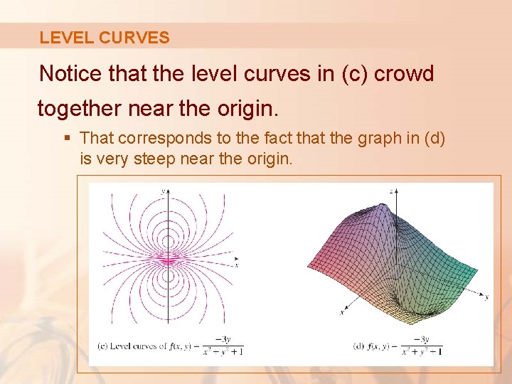
LEVEL CURVES The following figure shows some computer-generated level curves together with the corresponding computer-generated graphs.

LEVEL CURVES

LEVEL CURVES Notice that the level curves in (c) crowd together near the origin. § That corresponds to the fact that the graph in (d) is very steep near the origin.

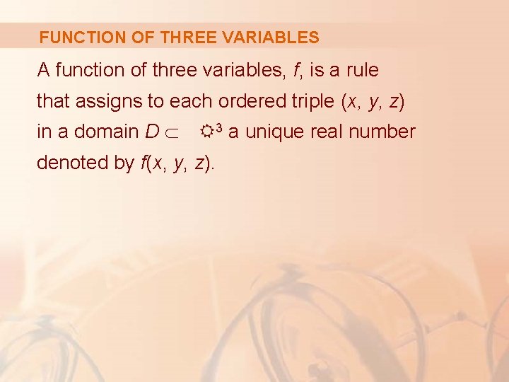
FUNCTION OF THREE VARIABLES A function of three variables, f, is a rule that assigns to each ordered triple (x, y, z) in a domain D R 3 a unique real number denoted by f(x, y, z).

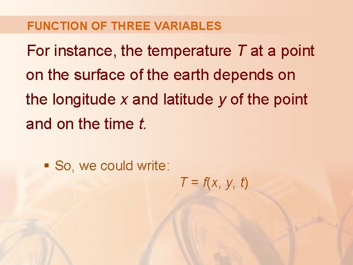
FUNCTION OF THREE VARIABLES For instance, the temperature T at a point on the surface of the earth depends on the longitude x and latitude y of the point and on the time t. § So, we could write: T = f(x, y, t)

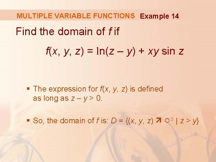
MULTIPLE VARIABLE FUNCTIONS Example 14 Find the domain of f if f(x, y, z) = ln(z – y) + xy sin z § The expression for f(x, y, z) is defined as long as z – y > 0. § So, the domain of f is: D = {(x, y, z) R 3 | z > y}

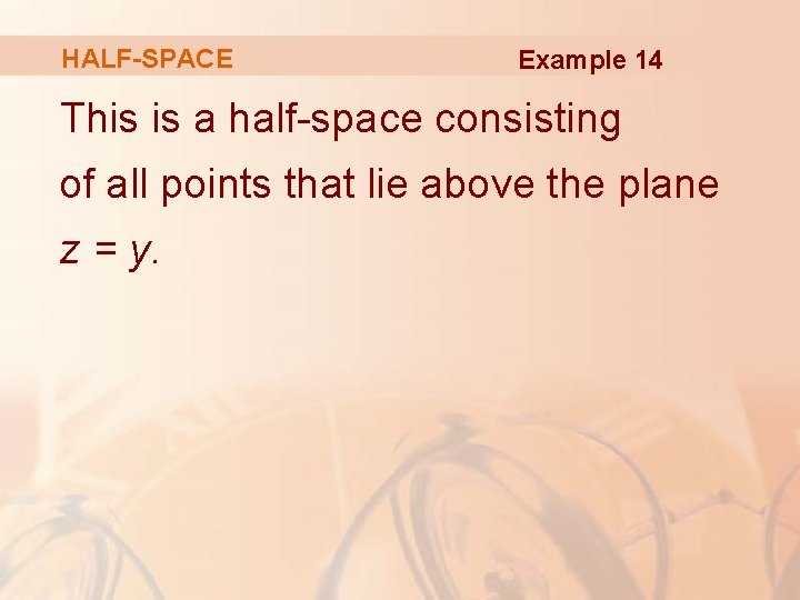
HALF-SPACE Example 14 This is a half-space consisting of all points that lie above the plane z = y.

MULTIPLE VARIABLE FUNCTIONS It’s very difficult to visualize a function f of three variables by its graph. § That would lie in a four-dimensional space.

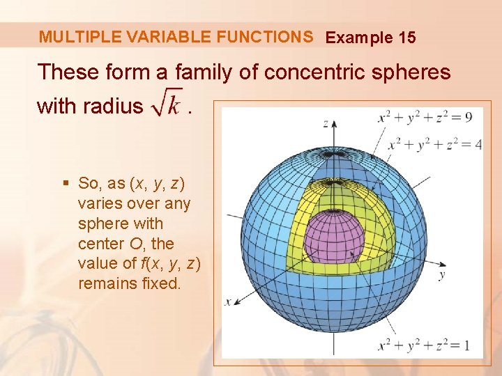
MULTIPLE VARIABLE FUNCTIONS However, we do gain some insight into f by examining its level surfaces—the surfaces with equations f(x, y, z) = k, where k is a constant. § If the point (x, y, z) moves along a level surface, the value of f(x, y, z) remains fixed.

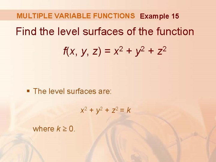
MULTIPLE VARIABLE FUNCTIONS Example 15 Find the level surfaces of the function f(x, y, z) = x 2 + y 2 + z 2 § The level surfaces are: x 2 + y 2 + z 2 = k where k ≥ 0.

MULTIPLE VARIABLE FUNCTIONS Example 15 These form a family of concentric spheres with radius . § So, as (x, y, z) varies over any sphere with center O, the value of f(x, y, z) remains fixed.

MULTIPLE VARIABLE FUNCTIONS Functions of any number of variables can be considered. § A function of n variables is a rule that assigns a number z = f(x 1, x 2, . . . , xn) to an n-tuple (x 1, x 2, . . . , xn) of real numbers. § We denote Rn by the set of all such n-tuples.

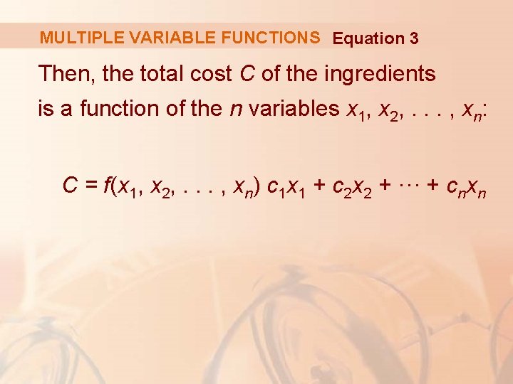
MULTIPLE VARIABLE FUNCTIONS For example, suppose, for making a food product in a company, § n different ingredients are used. § ci is the cost per unit of the ingredient. § xi units of the i th ingredient are used.

MULTIPLE VARIABLE FUNCTIONS Equation 3 Then, the total cost C of the ingredients is a function of the n variables x 1, x 2, . . . , xn: C = f(x 1, x 2, . . . , xn) c 1 x 1 + c 2 x 2 + ··· + cnxn

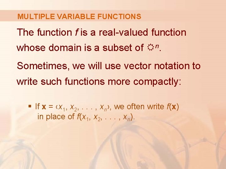
MULTIPLE VARIABLE FUNCTIONS The function f is a real-valued function whose domain is a subset of Rn. Sometimes, we will use vector notation to write such functions more compactly: § If x = ‹x 1, x 2, . . . , xn›, we often write f(x) in place of f(x 1, x 2, . . . , xn).

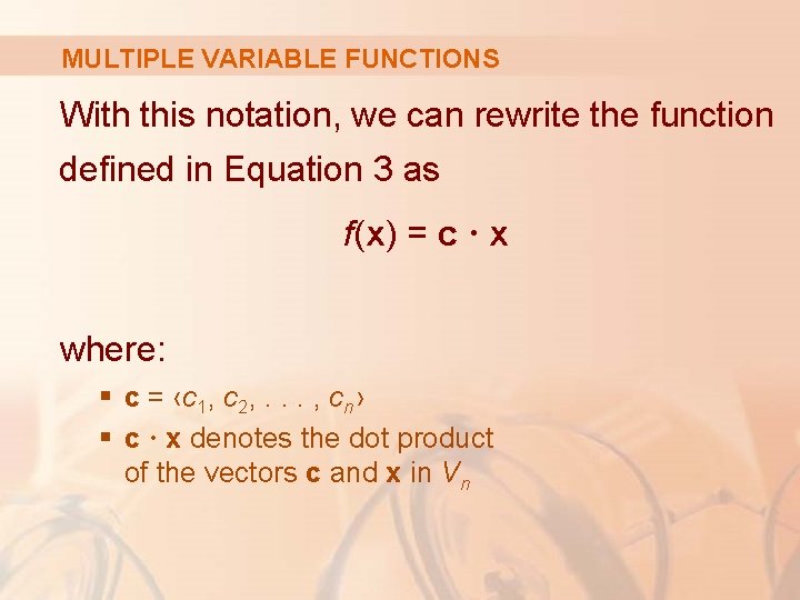
MULTIPLE VARIABLE FUNCTIONS With this notation, we can rewrite the function defined in Equation 3 as f(x) = c · x where: § c = ‹c 1, c 2, . . . , cn› § c · x denotes the dot product of the vectors c and x in Vn

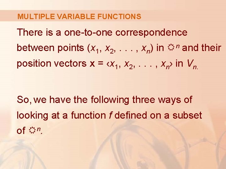
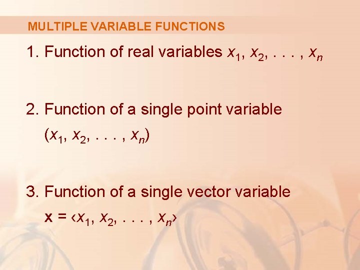
MULTIPLE VARIABLE FUNCTIONS There is a one-to-one correspondence between points (x 1, x 2, . . . , xn) in Rn and their position vectors x = ‹x 1, x 2, . . . , xn› in Vn. So, we have the following three ways of looking at a function f defined on a subset of Rn.

MULTIPLE VARIABLE FUNCTIONS 1. Function of real variables x 1, x 2, . . . , xn 2. Function of a single point variable (x 1, x 2, . . . , xn) 3. Function of a single vector variable x = ‹x 1, x 2, . . . , xn›

MULTIPLE VARIABLE FUNCTIONS We will see that all three points of view are useful.