14 Partial Derivatives Copyright Cengage Learning All rights

14 Partial Derivatives Copyright © Cengage Learning. All rights reserved.

14. 8 Lagrange Multipliers Copyright © Cengage Learning. All rights reserved.

Lagrange Multipliers In this section we present Lagrange’s method for maximizing or minimizing a general function f (x, y, z) subject to a constraint (or side condition) of the form g(x, y, z) = k. It’s easier to explain the geometric basis of Lagrange’s method for functions of two variables. So we start by trying to find the extreme values of f (x, y) subject to a constraint of the form g(x, y) = k. In other words, we seek the extreme values of f (x, y) when the point (x, y) is restricted to lie on the level curve g(x, y) = k. 3

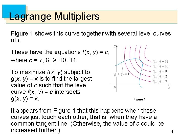
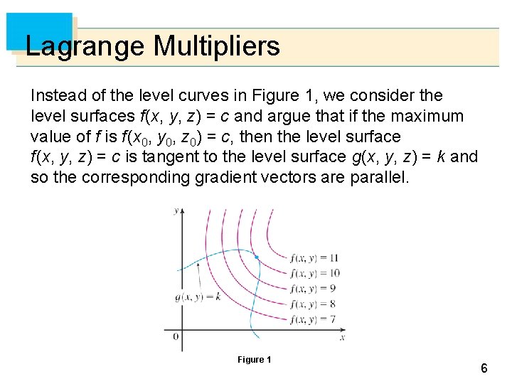
Lagrange Multipliers Figure 1 shows this curve together with several level curves of f. These have the equations f (x, y) = c, where c = 7, 8, 9, 10, 11. To maximize f (x, y) subject to g(x, y) = k is to find the largest value of c such that the level curve f (x, y) = c intersects g(x, y) = k. Figure 1 It appears from Figure 1 that this happens when these curves just touch each other, that is, when they have a common tangent line. (Otherwise, the value of c could be increased further. ) 4

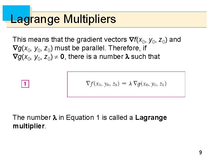
Lagrange Multipliers This means that the normal lines at the point (x 0, y 0) where they touch are identical. So the gradient vectors are parallel; that is, f (x 0, y 0) = g(x 0, y 0) for some scalar . This kind of argument also applies to the problem of finding the extreme values of f (x, y, z) subject to the constraint g(x, y, z) = k. Thus the point (x, y, z) is restricted to lie on the level surface S with equation g(x, y, z) = k. 5

Lagrange Multipliers Instead of the level curves in Figure 1, we consider the level surfaces f (x, y, z) = c and argue that if the maximum value of f is f (x 0, y 0, z 0) = c, then the level surface f (x, y, z) = c is tangent to the level surface g(x, y, z) = k and so the corresponding gradient vectors are parallel. Figure 1 6

Lagrange Multipliers This intuitive argument can be made precise as follows. Suppose that a function f has an extreme value at a point P(x 0, y 0, z 0) on the surface S and let C be a curve with vector equation r(t) = x(t), y(t), z(t) that lies on S and passes through P. If t 0 is the parameter value corresponding to the point P, then r(t 0) = x 0, y 0, z 0. The composite function h(t) = f (x(t), y(t), z(t)) represents the values that f takes on the curve C. 7

Lagrange Multipliers Since f has an extreme value at (x 0, y 0, z 0), it follows that h has an extreme value at t 0, so h (t 0) = 0. But if f is differentiable, we can use the Chain Rule to write 0 = h (t 0) = fx(x 0, y 0, z 0)x (t 0) + fy(x 0, y 0, z 0)y (t 0) + fz(x 0, y 0, z 0)z (t 0) = f (x 0, y 0, z 0) r (t 0) This shows that the gradient vector f (x 0, y 0, z 0) is orthogonal to the tangent vector r (t 0) to every such curve C. But we already know that the gradient vector of g, g(x 0, y 0, z 0), is also orthogonal to r (t 0) for every such curve. 8

Lagrange Multipliers This means that the gradient vectors f (x 0, y 0, z 0) and g(x 0, y 0, z 0) must be parallel. Therefore, if g(x 0, y 0, z 0) 0, there is a number such that The number in Equation 1 is called a Lagrange multiplier. 9

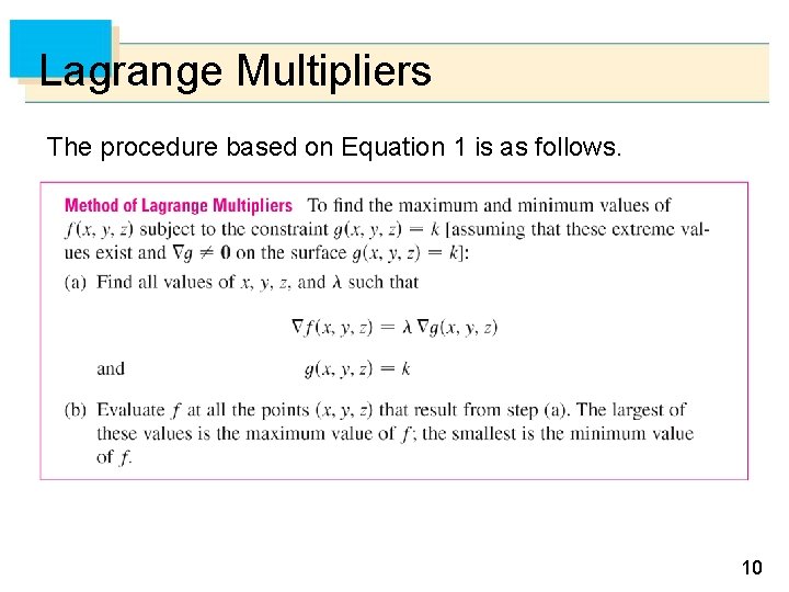
Lagrange Multipliers The procedure based on Equation 1 is as follows. 10

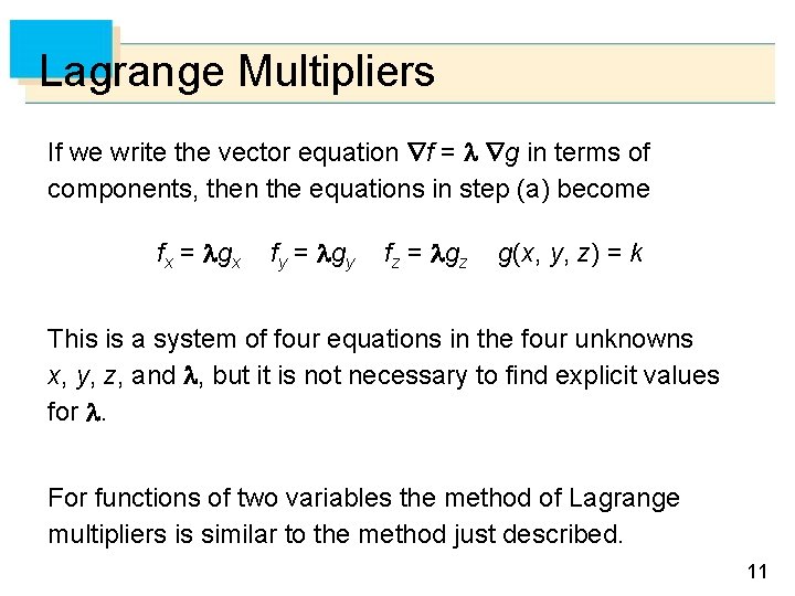
Lagrange Multipliers If we write the vector equation f = g in terms of components, then the equations in step (a) become fx = gx fy = gy fz = gz g(x, y, z) = k This is a system of four equations in the four unknowns x, y, z, and , but it is not necessary to find explicit values for . For functions of two variables the method of Lagrange multipliers is similar to the method just described. 11

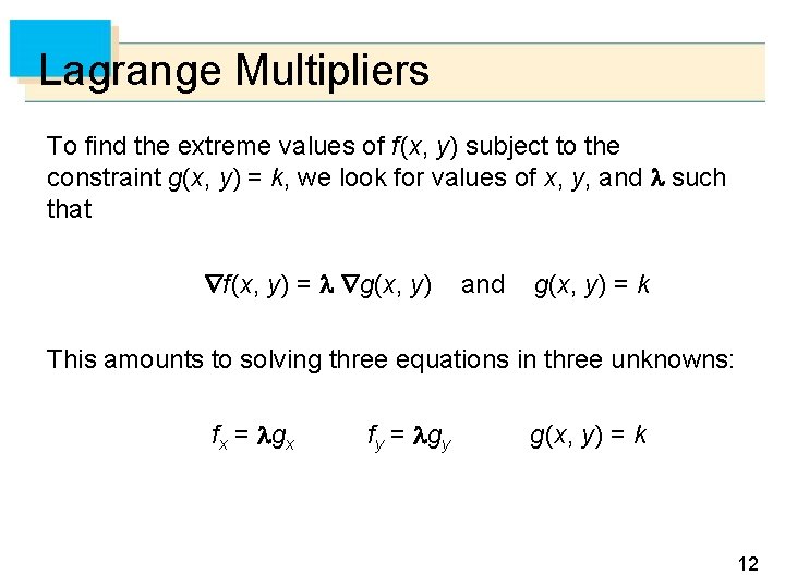
Lagrange Multipliers To find the extreme values of f (x, y) subject to the constraint g(x, y) = k, we look for values of x, y, and such that f (x, y) = g(x, y) and g(x, y) = k This amounts to solving three equations in three unknowns: fx = gx fy = gy g(x, y) = k 12

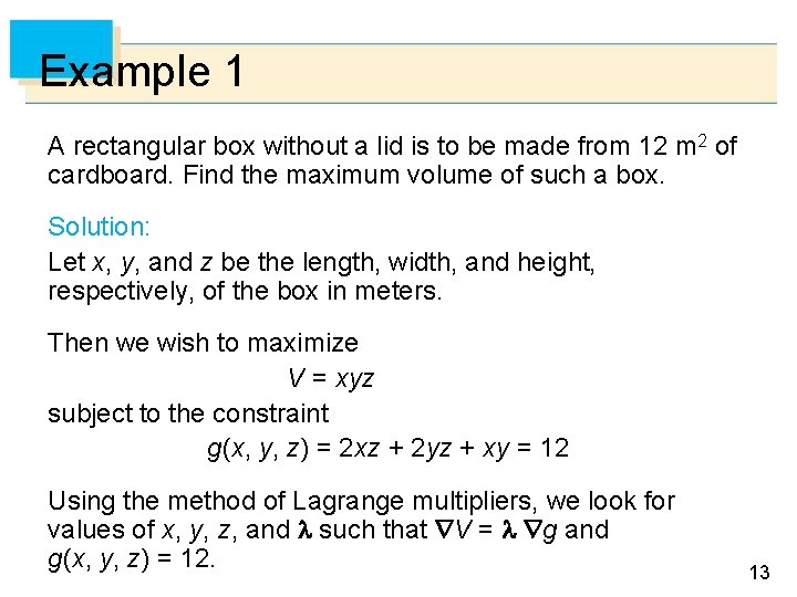
Example 1 A rectangular box without a lid is to be made from 12 m 2 of cardboard. Find the maximum volume of such a box. Solution: Let x, y, and z be the length, width, and height, respectively, of the box in meters. Then we wish to maximize V = xyz subject to the constraint g(x, y, z) = 2 xz + 2 yz + xy = 12 Using the method of Lagrange multipliers, we look for values of x, y, z, and such that V = g and g(x, y, z) = 12. 13

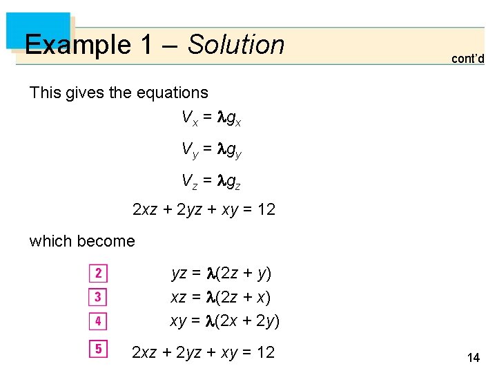
Example 1 – Solution cont’d This gives the equations Vx = gx Vy = gy Vz = gz 2 xz + 2 yz + xy = 12 which become yz = (2 z + y) xz = (2 z + x) xy = (2 x + 2 y) 2 xz + 2 yz + xy = 12 14

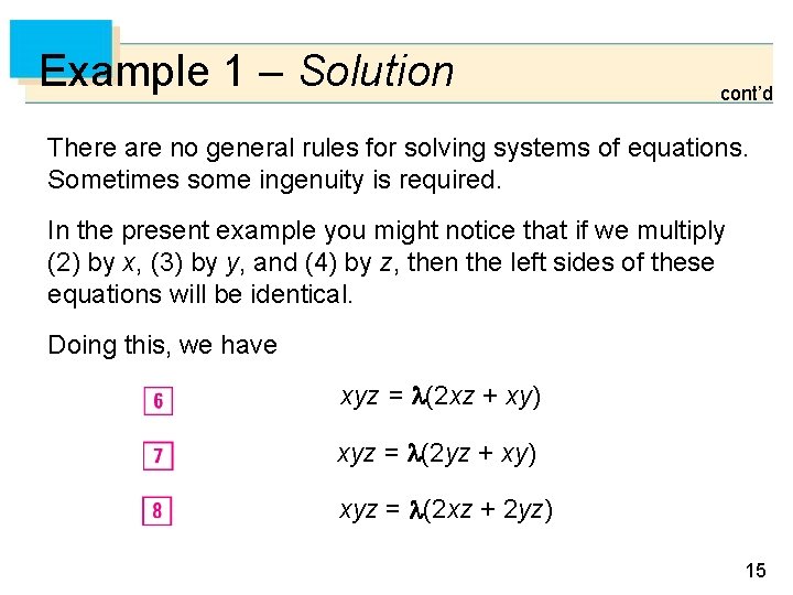
Example 1 – Solution cont’d There are no general rules for solving systems of equations. Sometimes some ingenuity is required. In the present example you might notice that if we multiply (2) by x, (3) by y, and (4) by z, then the left sides of these equations will be identical. Doing this, we have xyz = (2 xz + xy) xyz = (2 yz + xy) xyz = (2 xz + 2 yz) 15

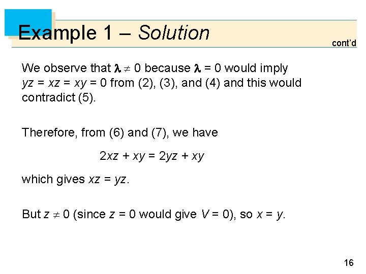
Example 1 – Solution cont’d We observe that 0 because = 0 would imply yz = xy = 0 from (2), (3), and (4) and this would contradict (5). Therefore, from (6) and (7), we have 2 xz + xy = 2 yz + xy which gives xz = yz. But z 0 (since z = 0 would give V = 0), so x = y. 16

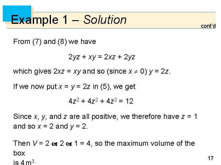
Example 1 – Solution cont’d From (7) and (8) we have 2 yz + xy = 2 xz + 2 yz which gives 2 xz = xy and so (since x 0) y = 2 z. If we now put x = y = 2 z in (5), we get 4 z 2 + 4 z 2 = 12 Since x, y, and z are all positive, we therefore have z = 1 and so x = 2 and y = 2. Then V = 2 2 1 = 4, so the maximum volume of the box 3. 17

Two Constraints 18

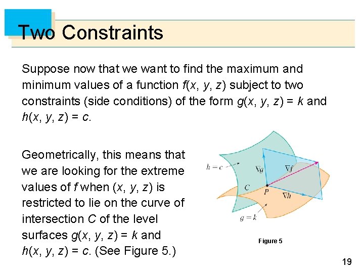
Two Constraints Suppose now that we want to find the maximum and minimum values of a function f (x, y, z) subject to two constraints (side conditions) of the form g(x, y, z) = k and h(x, y, z) = c. Geometrically, this means that we are looking for the extreme values of f when (x, y, z) is restricted to lie on the curve of intersection C of the level surfaces g(x, y, z) = k and h(x, y, z) = c. (See Figure 5. ) Figure 5 19

Two Constraints Suppose f has such an extreme value at a point P(x 0, y 0, z 0). We know from the beginning of this section that f is orthogonal to C at P. But we also know that g is orthogonal to g(x, y, z) = k and h is orthogonal to h(x, y, z) = c, so g and h are both orthogonal to C. This means that the gradient vector f (x 0, y 0, z 0) is in the plane determined by g(x 0, y 0, z 0) and h(x 0, y 0, z 0). (We assume that these gradient vectors are not zero and not parallel. ) 20

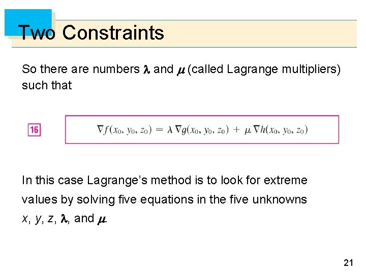
Two Constraints So there are numbers and (called Lagrange multipliers) such that In this case Lagrange’s method is to look for extreme values by solving five equations in the five unknowns x, y, z, , and . 21

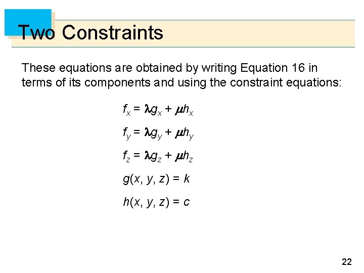
Two Constraints These equations are obtained by writing Equation 16 in terms of its components and using the constraint equations: fx = gx + hx fy = gy + hy fz = gz + hz g(x, y, z) = k h(x, y, z) = c 22

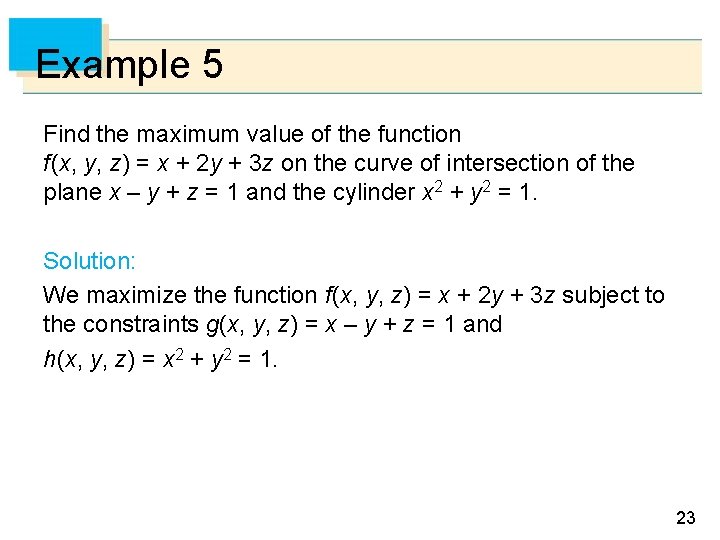
Example 5 Find the maximum value of the function f (x, y, z) = x + 2 y + 3 z on the curve of intersection of the plane x – y + z = 1 and the cylinder x 2 + y 2 = 1. Solution: We maximize the function f (x, y, z) = x + 2 y + 3 z subject to the constraints g(x, y, z) = x – y + z = 1 and h(x, y, z) = x 2 + y 2 = 1. 23

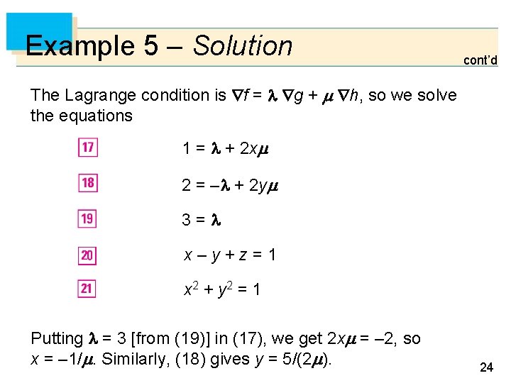
Example 5 – Solution cont’d The Lagrange condition is f = g + h, so we solve the equations 1 = + 2 x 2 = – + 2 y 3= x–y+z=1 x 2 + y 2 = 1 Putting = 3 [from (19)] in (17), we get 2 x = – 2, so x = – 1/. Similarly, (18) gives y = 5/(2 ). 24

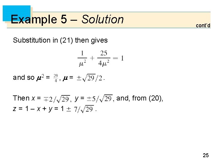
Example 5 – Solution cont’d Substitution in (21) then gives and so 2 = , = Then x = z=1–x+y=1 . y= and, from (20), . 25

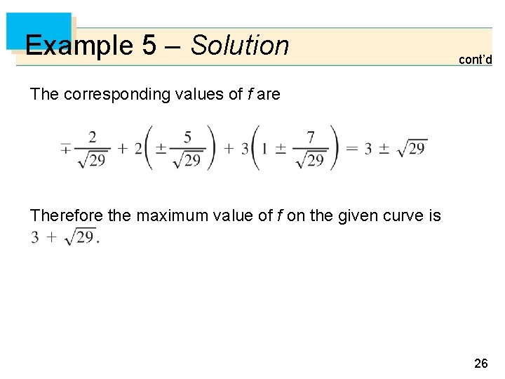
Example 5 – Solution cont’d The corresponding values of f are Therefore the maximum value of f on the given curve is 26