14 Evaluating Relational Operators v v v v

14. Evaluating Relational Operators v v v v v Table Statistics Operators and example schema Selection Projection Equijoins General Joins Set Operators Buffering Intergalactic standard reference § G. Graefe, "Query Evaluation Techniques for Large Databases, " ACM Computing Surveys, 25(2) (1993), pp. 73 -170 11/27/2020 PSU’s CS 587 1

Learning Objectives In a typical major DBMS, what statistics are automatically collected and when? v Given collected statistics, estimate a predicate’s output size/selectivity. v For each relational operator, describe the major algorithms, their optimizations, their pros and cons, and their costs v § § § 11/27/2020 Selection Projection Equijoins General Joins Set Operators PSU’s CS 587 2

Motivation/Review Assume Sailors has an index on age. v Does the optimal plan for this query use the index? SELECT * FROM Sailors S WHERE S. age < 31 v Moral: In order to choose the optimal plan we need to know the selectivity of the predicate/size of the output. v 11/27/2020 PSU’s CS 587 3

Collecting Statistics v What are statistics § Table sizes, index sizes, ranges of values, etc. v v Where are statistics kept? In the system catalog. Why collect statistics? § Statistics are needed to determine selectivity of predicates and sizes of outputs of operators. § Data in the previous bullet is needed to calculate costs of plans. § Data in the previous bullet is needed by the optimizer to find the optimal plan. v How often are statistics collected? § Typically done when 10% of the data has been updated. • Can be overidden manually • UPDATE STATISTICS, ANALYZE § Typically done by sampling, if table is large v Which tables/columns are monitored? § Typically all tables/columns are monitored 11/27/2020 PSU’s CS 587 4

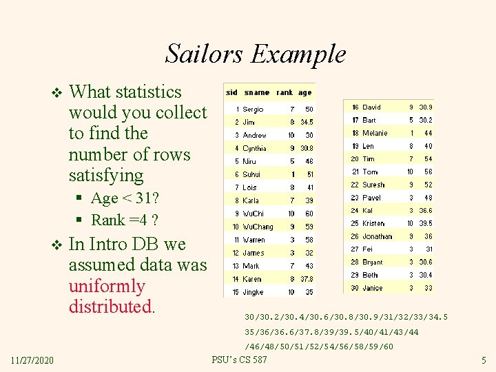
Sailors Example v What statistics would you collect to find the number of rows satisfying § Age < 31? § Rank =4 ? v In Intro DB we assumed data was uniformly distributed. 30/30. 2/30. 4/30. 6/30. 8/30. 9/31/32/33/34. 5 35/36/36. 6/37. 8/39/39. 5/40/41/43/44 /46/48/50/51/52/54/56/58/59/60 11/27/2020 PSU’s CS 587 5

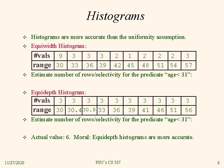
Histograms v v Histograms are more accurate than the uniformity assumption. Equiwidth Histogram: #vals 9 range 30 v 3 3 3 2 1 2 2 2 3 33 36 39 42 45 48 51 54 57 Estimate number of rows/selectivity for the predicate “age< 31”: v Equidepth Histogram: #vals 3 3 3 3 3 range 30 30. 430. 9 33 36 39 41 46 51 56 Estimate number of rows/selectivity for the predicate “age< 31”: v Actual value: 6. Moral: Equidepth histograms are more accurate. v 11/27/2020 PSU’s CS 587 6

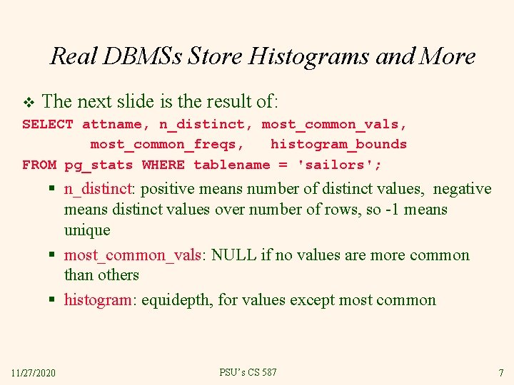
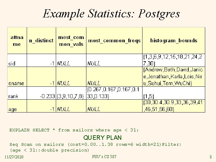
Real DBMSs Store Histograms and More v The next slide is the result of: SELECT attname, n_distinct, most_common_vals, most_common_freqs, histogram_bounds FROM pg_stats WHERE tablename = 'sailors'; § n_distinct: positive means number of distinct values, negative means distinct values over number of rows, so -1 means unique § most_common_vals: NULL if no values are more common than others § histogram: equidepth, for values except most common 11/27/2020 PSU’s CS 587 7

Example Statistics: Postgres EXPLAIN SELECT * from sailors where age < 31; QUERY PLAN Seq Scan on sailors (cost=0. 00. . 1. 38 rows=6 width=21)Filter: (age < 31: : double precision) 11/27/2020 PSU’s CS 587 8

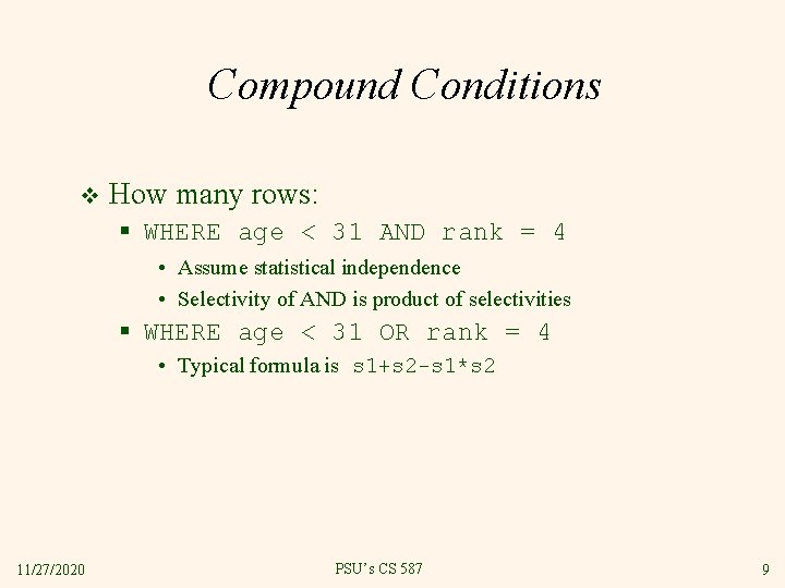
Compound Conditions v How many rows: § WHERE age < 31 AND rank = 4 • Assume statistical independence • Selectivity of AND is product of selectivities § WHERE age < 31 OR rank = 4 • Typical formula is s 1+s 2 -s 1*s 2 11/27/2020 PSU’s CS 587 9

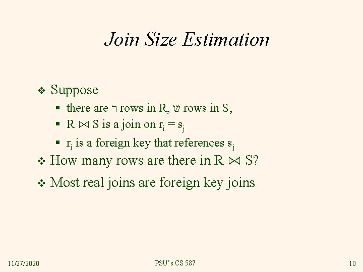
Join Size Estimation v Suppose § there are ר rows in R, ש rows in S, § R ⋈ S is a join on ri = sj § ri is a foreign key that references sj v How many rows are there in R ⋈ S? v Most real joins are foreign key joins 11/27/2020 PSU’s CS 587 10

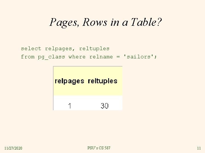
Pages, Rows in a Table? select relpages, reltuples from pg_class where relname = 'sailors'; 11/27/2020 PSU’s CS 587 11

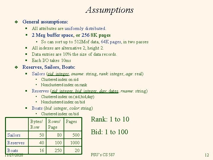
Assumptions v General assumptions: § All attributes are uniformly distributed. § 2 Meg buffer space, or 256 8 K pages • So can sort up to 512 Mof data, 64 K pages, in two passes § All indexes are alternative 2, height 2. § Data entries are 10% the size of data records. § Each I/O takes 10 ms v Reserves, Sailors, Boats: § Sailors (sid: integer, sname: string, rank: integer, age: real) • Clustered index on sid • Nonclustered index on rank § Reserves (sid: integer, bid: integer, day: dates, rname: string) • Clustered index on (sid, bid, day) • Nonclustered index on bid § Boats (bid: integer, color: string) • Clustered index on bid Bytes/ Rows/ Page Sailors 50 80 500 Reserves 40 1000 Boats 16 250 20 11/27/2020 Pages Rank: 1 to 10 Bid: 1 to 100 PSU’s CS 587 12

14. Evaluating Relational Operators and example schema v Selection v § One term § Nonclustered index optimization § Multiple terms Projection v Equijoins v General Joins v Set Operators v Buffering v 11/27/2020 PSU’s CS 587 13

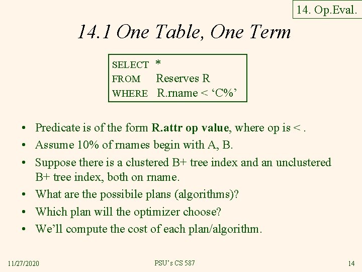
14. Op. Eval. 14. 1 One Table, One Term SELECT FROM WHERE * Reserves R R. rname < ‘C%’ • Predicate is of the form R. attr op value, where op is <. • Assume 10% of rnames begin with A, B. • Suppose there is a clustered B+ tree index and an unclustered B+ tree index, both on rname. • What are the possibile plans (algorithms)? • Which plan will the optimizer choose? • We’ll compute the cost of each plan/algorithm. 11/27/2020 PSU’s CS 587 14

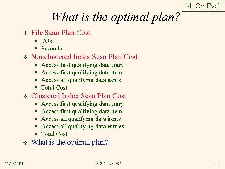
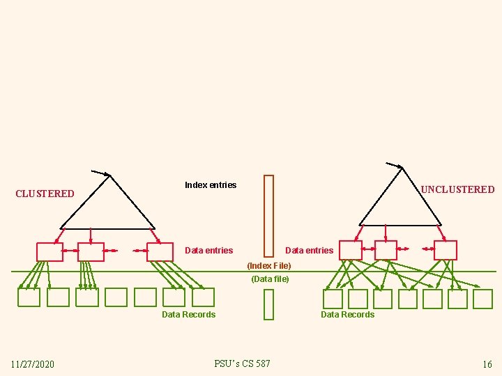
What is the optimal plan? v 14. Op. Eval. File Scan Plan Cost § I/Os § Seconds v Nonclustered Index Scan Plan Cost § § v Clustered Index Scan Plan Cost § § § v 11/27/2020 Access first qualifying data entry Access first qualifying data item Access all qualifying data items Total Cost Access first qualifying data entry Access first qualifying data item Access all qualifying data items Access all qualifying data entries Total Cost What is the optimal plan? PSU’s CS 587 15

CLUSTERED Index entries UNCLUSTERED Data entries (Index File) (Data file) Data Records 11/27/2020 PSU’s CS 587 Data Records 16

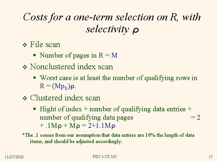
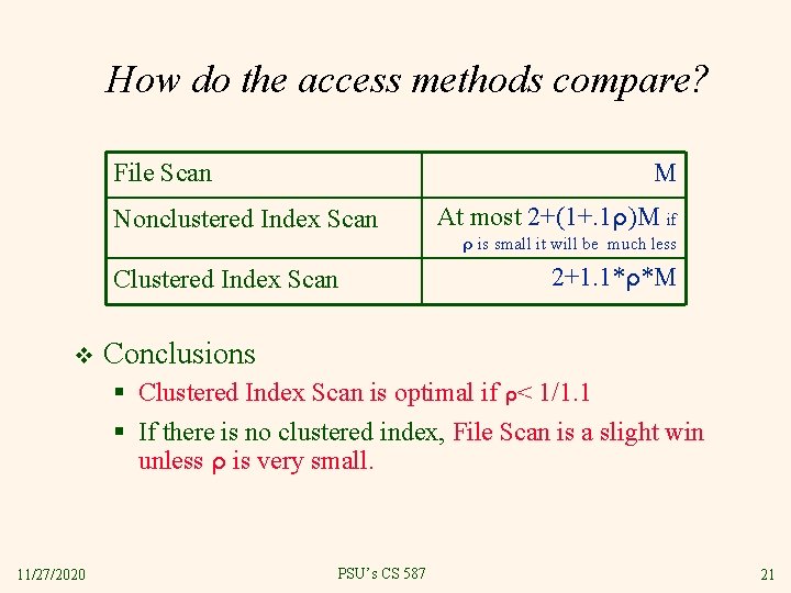
Costs for a one-term selection on R, with selectivity ρ v File scan § Number of pages in R = M v Nonclustered index scan § Worst case is at least the number of qualifying rows in R = (Mp. R)ρ. v Clustered index scan § Hight of index + number of qualifying data entries + number of qualifying data pages =2 +. 1 Mρ + Mρ = 2+1. 1 Mρ *The. 1 comes from our assumption that data entries are 10% the length of data items, and should be adjusted accordingly. 11/27/2020 PSU’s CS 587 17

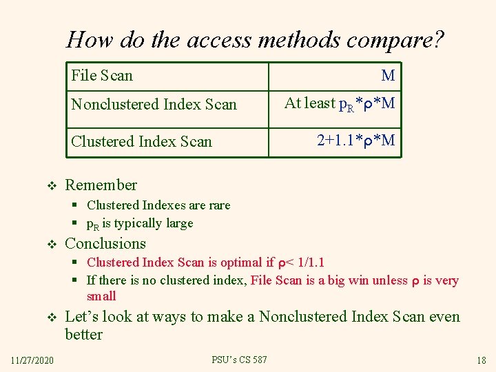
How do the access methods compare? File Scan M Nonclustered Index Scan Clustered Index Scan v At least p. R*ρ*M 2+1. 1*ρ*M Remember § Clustered Indexes are rare § p. R is typically large v Conclusions § Clustered Index Scan is optimal if ρ< 1/1. 1 § If there is no clustered index, File Scan is a big win unless ρ is very small v 11/27/2020 Let’s look at ways to make a Nonclustered Index Scan even better PSU’s CS 587 18

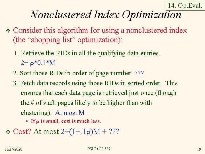
14. Op. Eval. Nonclustered Index Optimization v Consider this algorithm for using a nonclustered index (the “shopping list” optimization): 1. Retrieve the RIDs in all the qualifying data entries. 2+ ρ*0. 1*M 2. Sort those RIDs in order of page number. ? ? ? 3. Fetch data records using those RIDs in sorted order. This ensures that each data page is retrieved just once (though the # of such pages likely to be higher than with clustering). At most M • If ρ is small, cost is much less. v Cost? At most 2+(1+. 1ρ)M + ? ? ? 11/27/2020 PSU’s CS 587 19

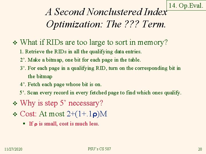
A Second Nonclustered Index Optimization: The ? ? ? Term. v 14. Op. Eval. What if RIDs are too large to sort in memory? 1. Retrieve the RIDs in all the qualifying data entries. 2’. Make a bitmap, one bit for each page in the table. 3’. For each page in a qualifying RID, turn on the corresponding bit in the bitmap 4’. Fetch each page whose bit is on. 5’. Scan every record in every fetched page to find which ones qualify. Why is step 5’ necessary? v Cost: At most 2+(1+. 1ρ)M v § If ρ is small, cost is much less. 11/27/2020 PSU’s CS 587 20

How do the access methods compare? File Scan M Nonclustered Index Scan At most 2+(1+. 1ρ)M if ρ is small it will be much less Clustered Index Scan v 2+1. 1*ρ*M Conclusions § Clustered Index Scan is optimal if ρ< 1/1. 1 § If there is no clustered index, File Scan is a slight win unless ρ is very small. 11/27/2020 PSU’s CS 587 21

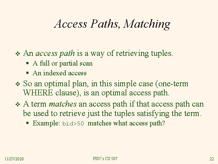
Access Paths, Matching v An access path is a way of retrieving tuples. § A full or partial scan § An indexed access So an optimal plan, in this simple case (one-term WHERE clause), is an optimal access path. v A term matches an access path if that access path can be used to retrieve just the tuples satisfying the term. v § Example: bid>50 matches what access path? 11/27/2020 PSU’s CS 587 22

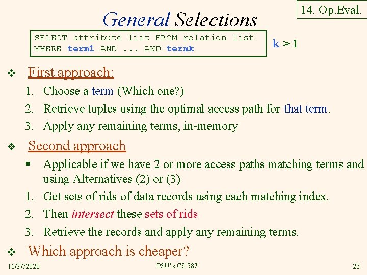
14. Op. Eval. General Selections SELECT attribute list FROM relation list WHERE term 1 AND. . . AND termk v k>1 First approach: 1. Choose a term (Which one? ) 2. Retrieve tuples using the optimal access path for that term. 3. Apply any remaining terms, in-memory v Second approach § Applicable if we have 2 or more access paths matching terms and using Alternatives (2) or (3) 1. Get sets of rids of data records using each matching index. 2. Then intersect these sets of rids 3. Retrieve the records and apply any remaining terms. v Which approach is cheaper? 11/27/2020 PSU’s CS 587 23

14. Evaluating Relational Operators and example schema v Selection v Projection v § What is the problem? § Sort and hash approaches Equijoins v General Joins v Set Operators v Buffering v 11/27/2020 PSU’s CS 587 24

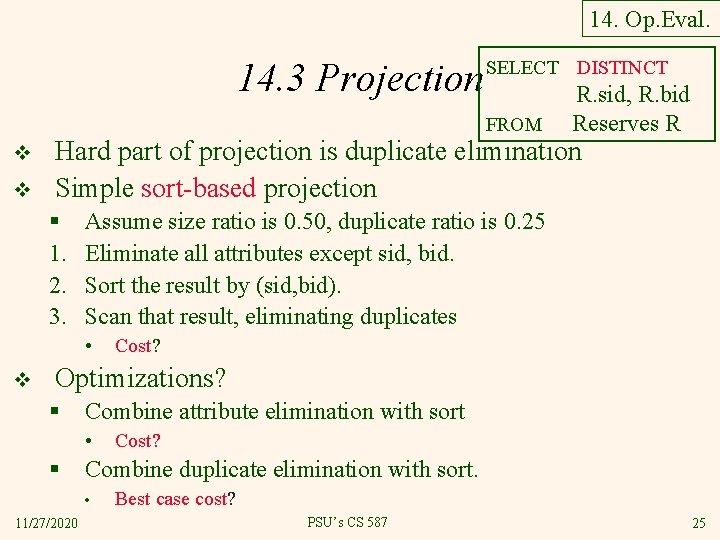
14. Op. Eval. 14. 3 Projection SELECT DISTINCT FROM v v Hard part of projection is duplicate elimination Simple sort-based projection § 1. 2. 3. Assume size ratio is 0. 50, duplicate ratio is 0. 25 Eliminate all attributes except sid, bid. Sort the result by (sid, bid). Scan that result, eliminating duplicates • v R. sid, R. bid Reserves R Cost? Optimizations? § Combine attribute elimination with sort • § Combine duplicate elimination with sort. • 11/27/2020 Cost? Best case cost? PSU’s CS 587 25

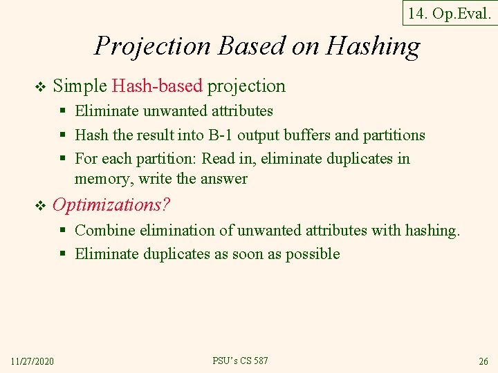
14. Op. Eval. Projection Based on Hashing v Simple Hash-based projection § Eliminate unwanted attributes § Hash the result into B-1 output buffers and partitions § For each partition: Read in, eliminate duplicates in memory, write the answer v Optimizations? § Combine elimination of unwanted attributes with hashing. § Eliminate duplicates as soon as possible 11/27/2020 PSU’s CS 587 26

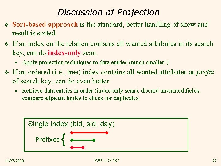
Discussion of Projection v v Sort-based approach is the standard; better handling of skew and result is sorted. If an index on the relation contains all wanted attributes in its search key, can do index-only scan. § v Apply projection techniques to data entries (much smaller!) If an ordered (i. e. , tree) index contains all wanted attributes as prefix of search key, can do even better: § Retrieve data entries in order (index-only scan), discard unwanted fields, compare adjacent tuples to check for duplicates. Single index (bid, sid, day) Prefixes 11/27/2020 { PSU’s CS 587 27

14. Evaluating Relational Operators v v Operators and example schema Selection Projection Equijoins § § § v v v 11/27/2020 Nested Loop Join Index Nested Loop Join Sort-Merge Join Hash Join Hybrid Hash Join General Joins Set Operators Buffering PSU’s CS 587 28

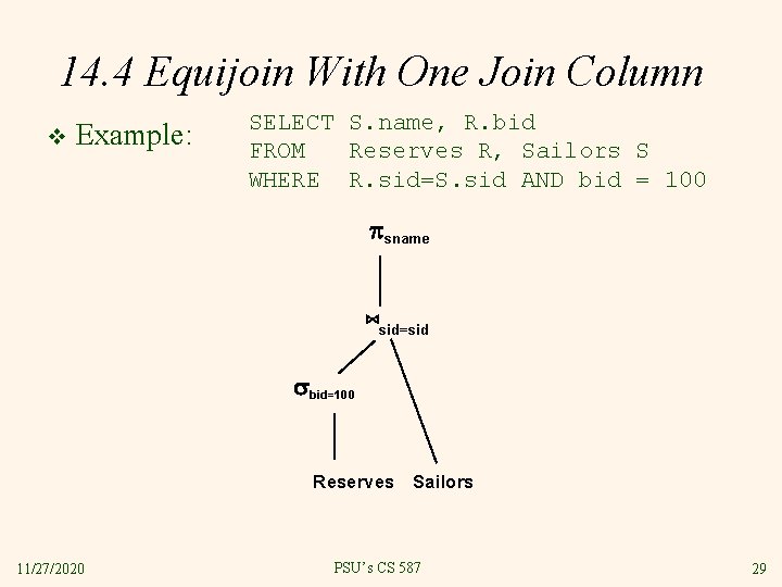
14. 4 Equijoin With One Join Column v Example: SELECT S. name, R. bid FROM Reserves R, Sailors S WHERE R. sid=S. sid AND bid = 100 sname ⋈sid=sid bid=100 Reserves Sailors 11/27/2020 PSU’s CS 587 29

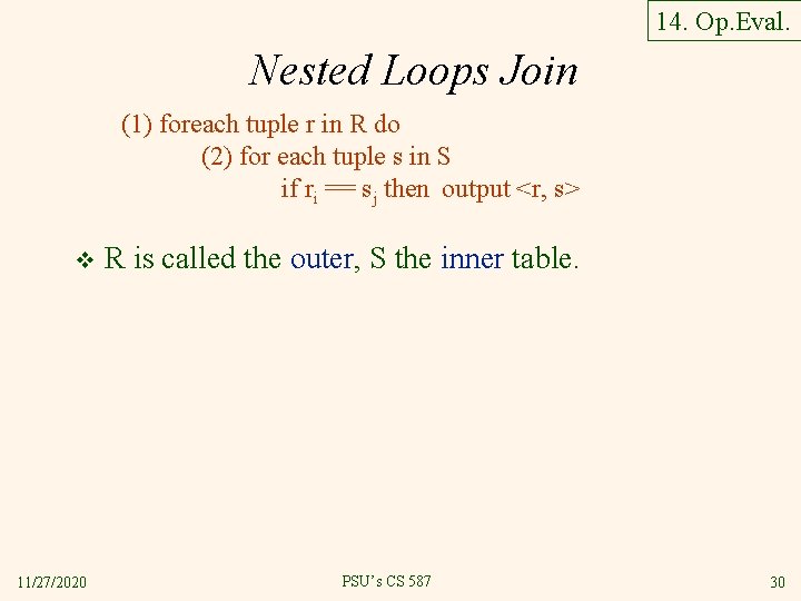
14. Op. Eval. Nested Loops Join (1) foreach tuple r in R do (2) for each tuple s in S if ri == sj then output <r, s> v 11/27/2020 R is called the outer, S the inner table. PSU’s CS 587 30

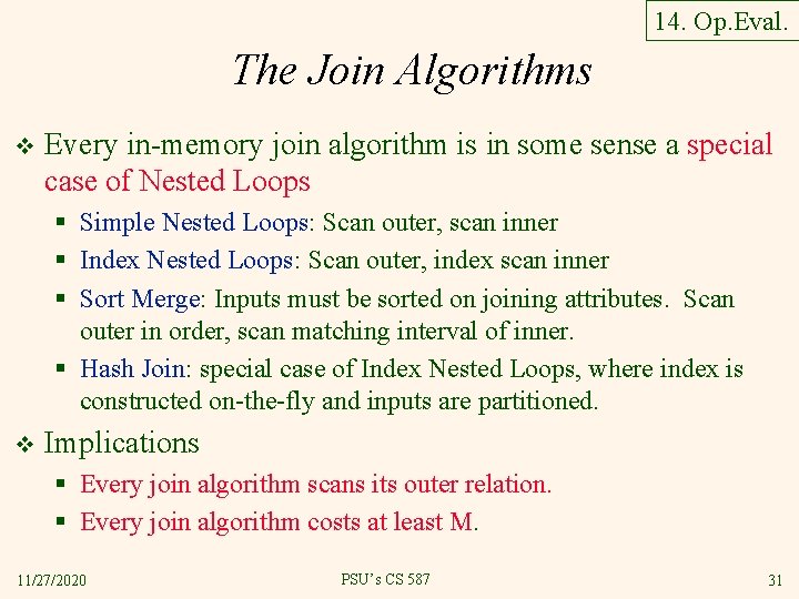
14. Op. Eval. The Join Algorithms v Every in-memory join algorithm is in some sense a special case of Nested Loops § Simple Nested Loops: Scan outer, scan inner § Index Nested Loops: Scan outer, index scan inner § Sort Merge: Inputs must be sorted on joining attributes. Scan outer in order, scan matching interval of inner. § Hash Join: special case of Index Nested Loops, where index is constructed on-the-fly and inputs are partitioned. v Implications § Every join algorithm scans its outer relation. § Every join algorithm costs at least M. 11/27/2020 PSU’s CS 587 31

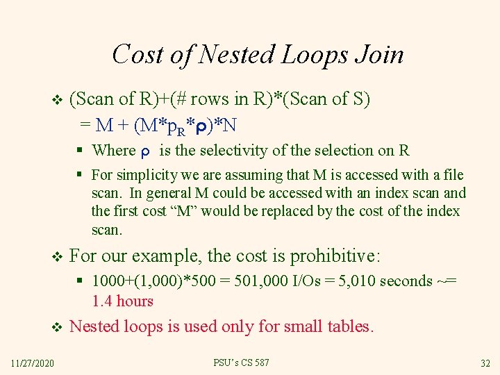
Cost of Nested Loops Join v (Scan of R)+(# rows in R)*(Scan of S) = M + (M*p. R*ρ)*N § Where ρ is the selectivity of the selection on R § For simplicity we are assuming that M is accessed with a file scan. In general M could be accessed with an index scan and the first cost “M” would be replaced by the cost of the index scan. v For our example, the cost is prohibitive: § 1000+(1, 000)*500 = 501, 000 I/Os = 5, 010 seconds ~= 1. 4 hours v 11/27/2020 Nested loops is used only for small tables. PSU’s CS 587 32

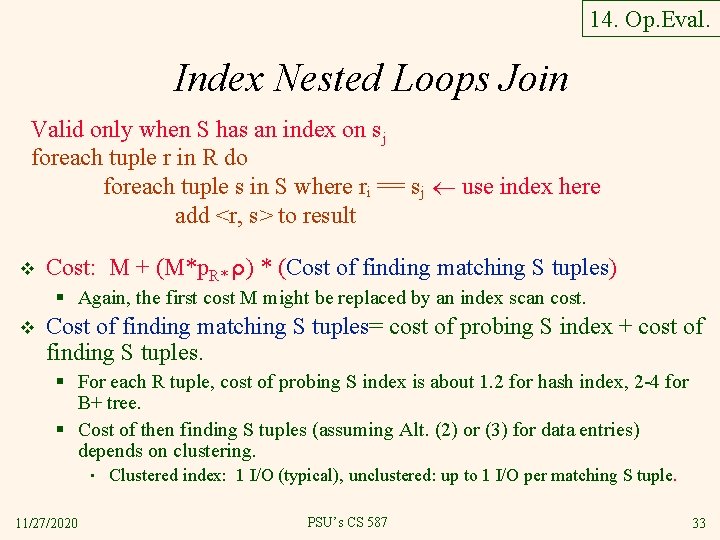
14. Op. Eval. Index Nested Loops Join Valid only when S has an index on sj foreach tuple r in R do foreach tuple s in S where ri == sj use index here add <r, s> to result v Cost: M + (M*p. R* ρ) * (Cost of finding matching S tuples) § Again, the first cost M might be replaced by an index scan cost. v Cost of finding matching S tuples= cost of probing S index + cost of finding S tuples. § For each R tuple, cost of probing S index is about 1. 2 for hash index, 2 -4 for B+ tree. § Cost of then finding S tuples (assuming Alt. (2) or (3) for data entries) depends on clustering. • 11/27/2020 Clustered index: 1 I/O (typical), unclustered: up to 1 I/O per matching S tuple. PSU’s CS 587 33

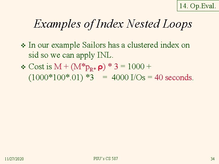
14. Op. Eval. Examples of Index Nested Loops In our example Sailors has a clustered index on sid so we can apply INL. v Cost is M + (M*p. R* ρ) * 3 = 1000 + (1000*100*. 01) *3 = 4000 I/Os = 40 seconds. v 11/27/2020 PSU’s CS 587 34

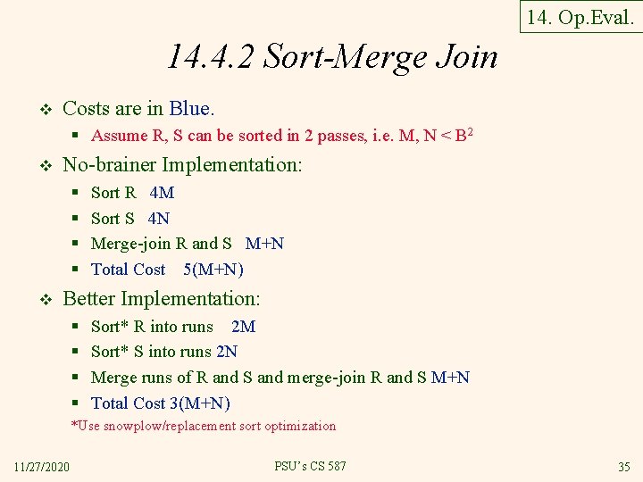
14. Op. Eval. 14. 4. 2 Sort-Merge Join v Costs are in Blue. § Assume R, S can be sorted in 2 passes, i. e. M, N < B 2 v No-brainer Implementation: § § v Sort R 4 M Sort S 4 N Merge-join R and S M+N Total Cost 5(M+N) Better Implementation: § § Sort* R into runs 2 M Sort* S into runs 2 N Merge runs of R and S and merge-join R and S M+N Total Cost 3(M+N) *Use snowplow/replacement sort optimization 11/27/2020 PSU’s CS 587 35

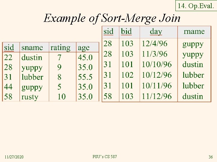
14. Op. Eval. Example of Sort-Merge Join 11/27/2020 PSU’s CS 587 36

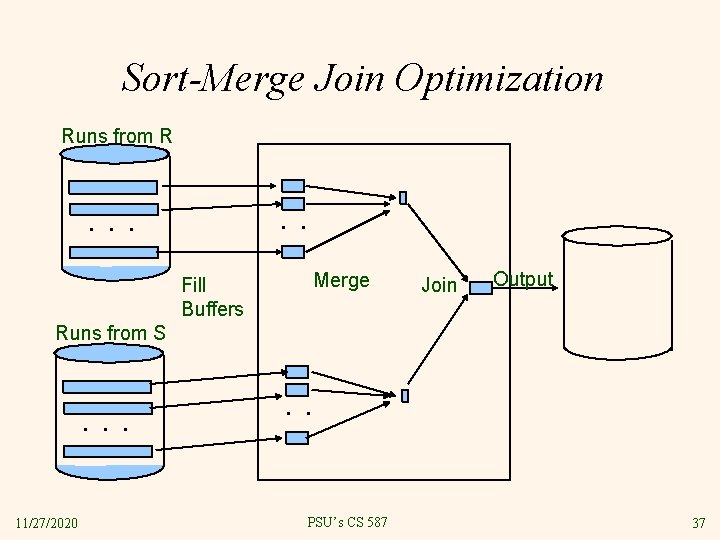
Sort-Merge Join Optimization Runs from R . . . Fill Buffers Merge Join Output Runs from S . . . 11/27/2020 . . PSU’s CS 587 37

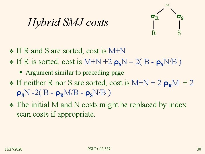
⋈ Hybrid SMJ costs R S R S If R and S are sorted, cost is M+N v If R is sorted, cost is M+N +2 ρSN – 2( B - ρSN/B ) v § Argument similar to preceding page v If neither R nor S are sorted, cost is M+N + 2 ρRM + 2 ρSN -2( B - ρRM/B - ρSN/B ) v The initial M and N costs might be replaced by index scan costs if appropriate. 11/27/2020 PSU’s CS 587 38

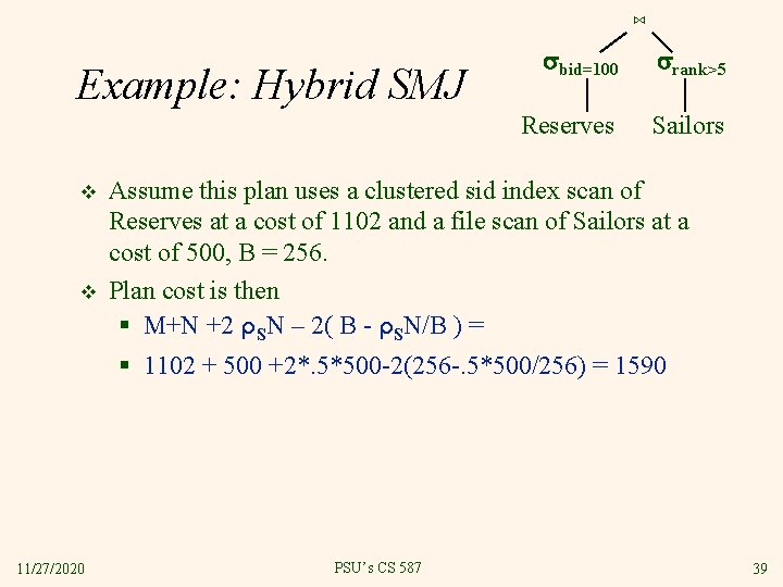
⋈ Example: Hybrid SMJ v v bid=100 rank>5 Reserves Sailors Assume this plan uses a clustered sid index scan of Reserves at a cost of 1102 and a file scan of Sailors at a cost of 500, B = 256. Plan cost is then § M+N +2 ρSN – 2( B - ρSN/B ) = § 1102 + 500 +2*. 5*500 -2(256 -. 5*500/256) = 1590 11/27/2020 PSU’s CS 587 39

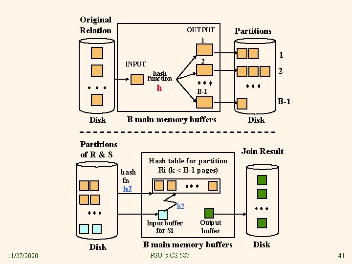
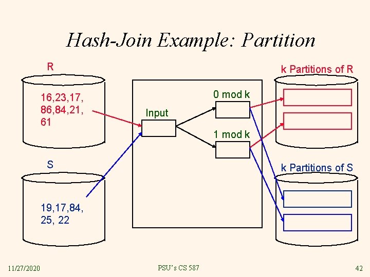
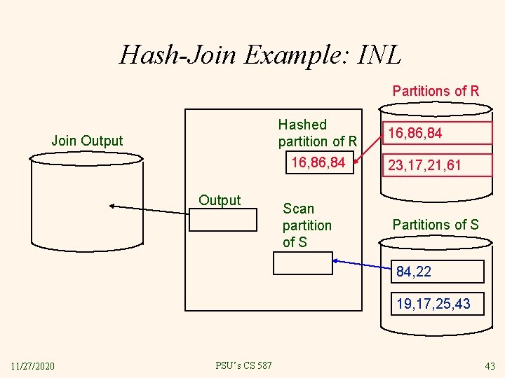
14. 4. 3 Hash-Join [677] v Confusing because it combines two distinct ideas: 1. Partition R and S using a hash function • You should understand how and why this works. Read the text if you don’t. 2. Join corresponding partitions using a version of INL with hash indexes built on-the-fly. • v The partition step could be followed by any join method in step 2. Hashing is used because § § § 11/27/2020 You should understand why the hash function used here must differ from the hash function used for partitioning. The tables are large (they needed partitioning) so NLJ is not a contender. The partitions were just created so they have no indexes on them, so classic INL is not possible. The partitions were just created so are not sorted, so SMJ is not a big winner. There may be cases where a sort order is needed later, but this is not considered. PSU’s CS 587 40

Original Relation OUTPUT 1 Partitions 1 2 INPUT 2 hash function . . . h B-1 Disk B main memory buffers Partitions of R & S Disk Join Result hash fn Hash table for partition Ri (k < B-1 pages) h 2 Input buffer for Si Disk 11/27/2020 Output buffer B main memory buffers PSU’s CS 587 Disk 41

Hash-Join Example: Partition R 16, 23, 17, 86, 84, 21, 61 k Partitions of R 0 mod k Input 1 mod k S k Partitions of S 19, 17, 84, 25, 22 11/27/2020 PSU’s CS 587 42

Hash-Join Example: INL Partitions of R Hashed partition of R 16, 84 Join Output Scan partition of S 16, 84 23, 17, 21, 61 Partitions of S 84, 22 19, 17, 25, 43 11/27/2020 PSU’s CS 587 43

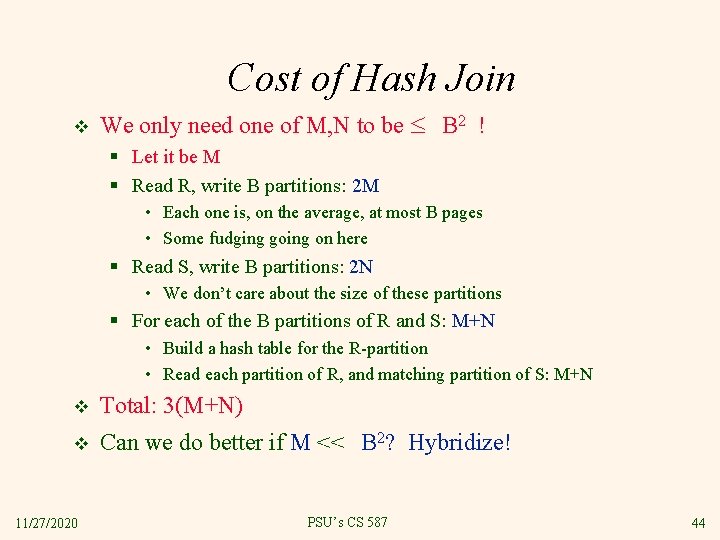
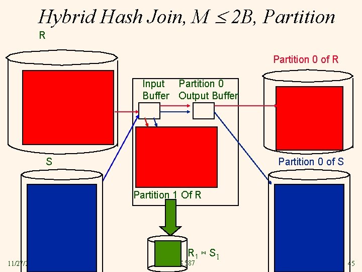
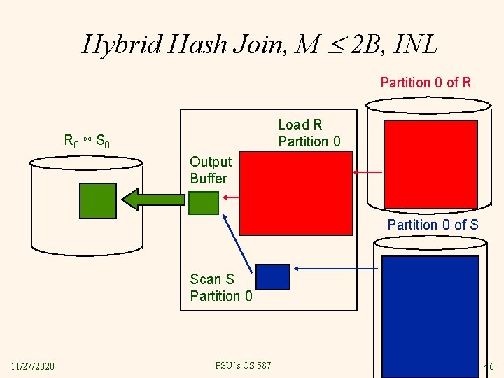
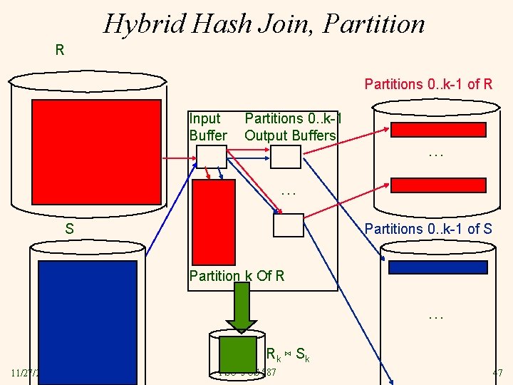
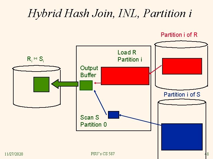
Cost of Hash Join v We only need one of M, N to be B 2 ! § Let it be M § Read R, write B partitions: 2 M • Each one is, on the average, at most B pages • Some fudging going on here § Read S, write B partitions: 2 N • We don’t care about the size of these partitions § For each of the B partitions of R and S: M+N • Build a hash table for the R-partition • Read each partition of R, and matching partition of S: M+N v Total: 3(M+N) v Can we do better if M << B 2? Hybridize! 11/27/2020 PSU’s CS 587 44

Hybrid Hash Join, M 2 B, Partition R Partition 0 of R Input Partition 0 Buffer Output Buffer S Partition 0 of S Partition 1 Of R 11/27/2020 R 1 ⋈ S 1 PSU’s CS 587 45

Hybrid Hash Join, M 2 B, INL Partition 0 of R Load R Partition 0 R 0 ⋈ S 0 Output Buffer Partition 0 of S Scan S Partition 0 11/27/2020 PSU’s CS 587 46

Hybrid Hash Join, Partition R Partitions 0. . k-1 of R Input Buffer Partitions 0. . k-1 Output Buffers … … S Partitions 0. . k-1 of S Partition k Of R … Rk ⋈ S k 11/27/2020 PSU’s CS 587 47

Hybrid Hash Join, INL, Partition i of R Load R Partition i Ri ⋈ S i Output Buffer Partition i of S Scan S Partition 0 11/27/2020 PSU’s CS 587 48

14. Op. Eval. Fudging in our treatment of Hash-Join If we build an in-memory hash table to speed up the matching of tuples, a little more memory is needed. v If the hash function does not partition uniformly, one or more R partitions may not fit in memory. v § In this case we can apply the hash-join technique recursively to do the join of this R-partition with its corresponding Spartition. 11/27/2020 PSU’s CS 587 49

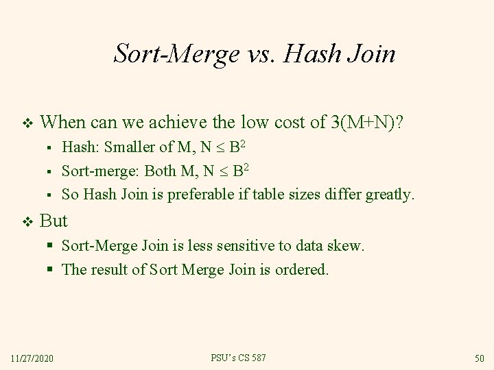
Sort-Merge vs. Hash Join v When can we achieve the low cost of 3(M+N)? § § § v Hash: Smaller of M, N B 2 Sort-merge: Both M, N B 2 So Hash Join is preferable if table sizes differ greatly. But § Sort-Merge Join is less sensitive to data skew. § The result of Sort Merge Join is ordered. 11/27/2020 PSU’s CS 587 50

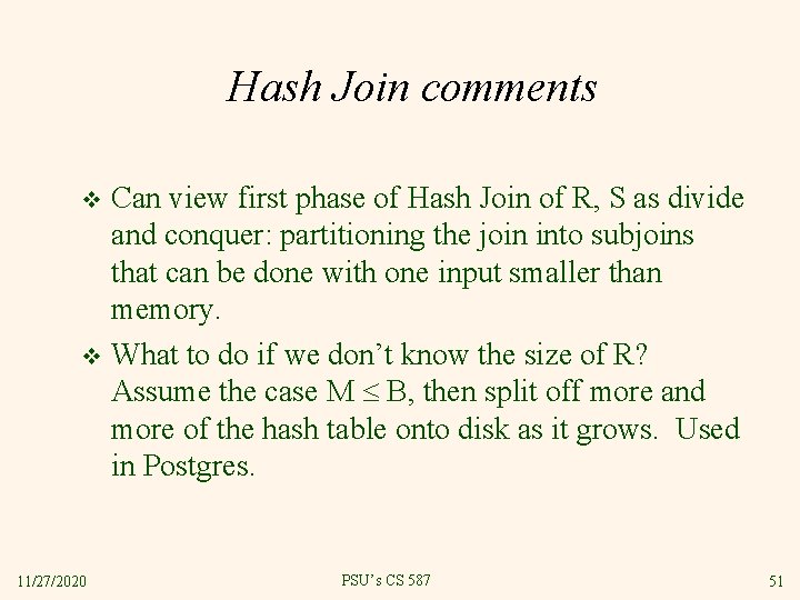
Hash Join comments Can view first phase of Hash Join of R, S as divide and conquer: partitioning the join into subjoins that can be done with one input smaller than memory. v What to do if we don’t know the size of R? Assume the case M B, then split off more and more of the hash table onto disk as it grows. Used in Postgres. v 11/27/2020 PSU’s CS 587 51

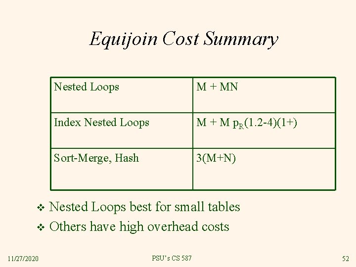
Equijoin Cost Summary Nested Loops M + MN Index Nested Loops M + M p. R(1. 2 -4)(1+) Sort-Merge, Hash 3(M+N) Nested Loops best for small tables v Others have high overhead costs v 11/27/2020 PSU’s CS 587 52

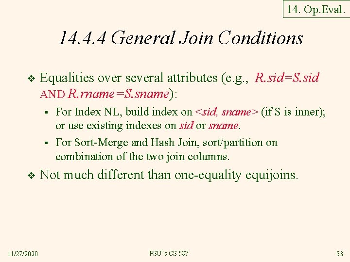
14. Op. Eval. 14. 4. 4 General Join Conditions v Equalities over several attributes (e. g. , R. sid=S. sid AND R. rname=S. sname): § § v 11/27/2020 For Index NL, build index on <sid, sname> (if S is inner); or use existing indexes on sid or sname. For Sort-Merge and Hash Join, sort/partition on combination of the two join columns. Not much different than one-equality equijoins. PSU’s CS 587 53

Inequality Conditions v Typical example: R. rname < S. sname § § Relatively rare. Does the example make sense? For Index NL, need (clustered!) B+ tree index to get any efficiency. • Range probes on inner; # matches likely to be much higher than for equality joins. § § 11/27/2020 Hash Join, Sort Merge Join not applicable. With no index, Block NL is the best join method. PSU’s CS 587 54

14. Op. Eval. 14. 5 Set Operations v INTERSECTION: § INTERSECTION is a special case of join. • How is it a special case? § So all the usual join algorithms apply v CROSS PRODUCT § Also a special case of join • How? § What join algorithm is best to compute CROSS PRODUCT? • Will Sort-Merge or Hash help? 11/27/2020 PSU’s CS 587 55

UNION and EXCEPT They are similar; we’ll do UNION. v The hard part is removing duplicates. v Sorting based approach to union: v § § § v Sort both relations (on a key). Merge sorted relations, discarding duplicates. Alternative: Merge runs from Pass 0 for both relations. Hash based approach to union: § § 11/27/2020 Partition R and S using hash function h. For each S-partition, build in-memory hash table, scan corresponding R-partition and add tuples to table while discarding duplicates. PSU’s CS 587 56

14. Op. Eval. 14. 6 Aggregates w/o grouping v Example § SELECT AVE(S. age) FROM SAILORS S v In general, requires scanning the relation. § v What is the cost for this query? Given index whose search key includes all attributes in the SELECT or WHERE clauses, can do index-only scan. § 11/27/2020 If there is an index on age, what is the cost of this query? PSU’s CS 587 57

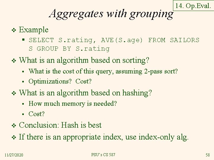
Aggregates with grouping v 14. Op. Eval. Example § SELECT S. rating, AVE(S. age) FROM SAILORS S GROUP BY S. rating v What is an algorithm based on sorting? § § v What is the cost of this query, assuming 2 -pass sort? Optimizations? Cost? What is an algorithm based on hashing? § § How much memory is needed? Cost? Conclusion: Hash is best v If there is an appropriate index, use index-only alg. v 11/27/2020 PSU’s CS 587 58

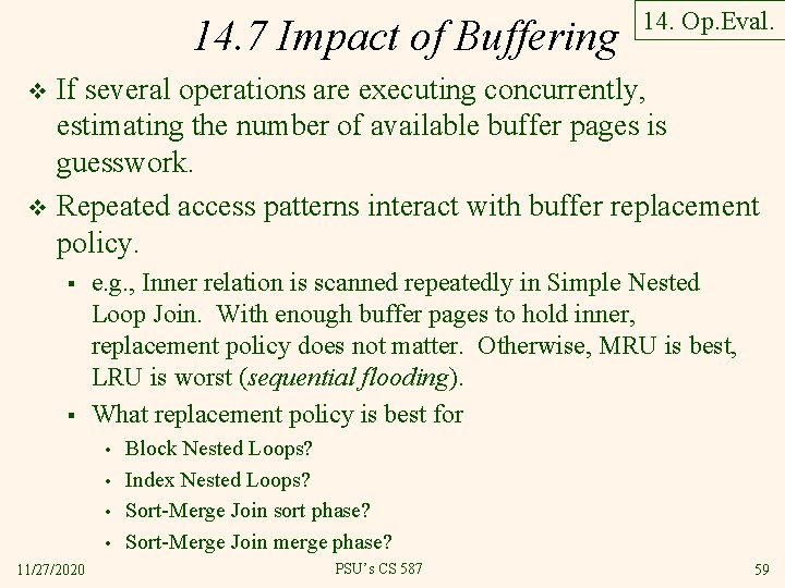
14. 7 Impact of Buffering 14. Op. Eval. If several operations are executing concurrently, estimating the number of available buffer pages is guesswork. v Repeated access patterns interact with buffer replacement policy. v § § e. g. , Inner relation is scanned repeatedly in Simple Nested Loop Join. With enough buffer pages to hold inner, replacement policy does not matter. Otherwise, MRU is best, LRU is worst (sequential flooding). What replacement policy is best for • • 11/27/2020 Block Nested Loops? Index Nested Loops? Sort-Merge Join sort phase? Sort-Merge Join merge phase? PSU’s CS 587 59