14 7 Maximum and Minimum Values Maximum and

14. 7 Maximum and Minimum Values

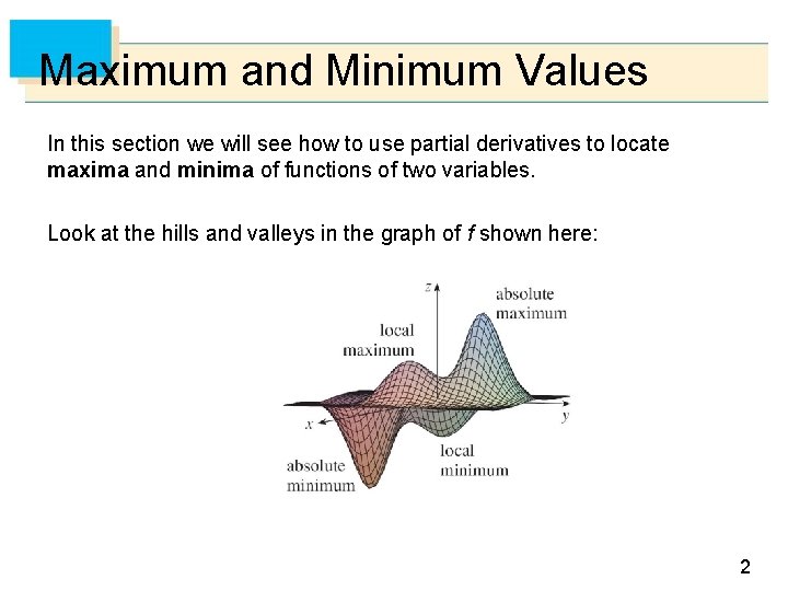
Maximum and Minimum Values In this section we will see how to use partial derivatives to locate maxima and minima of functions of two variables. Look at the hills and valleys in the graph of f shown here: 2

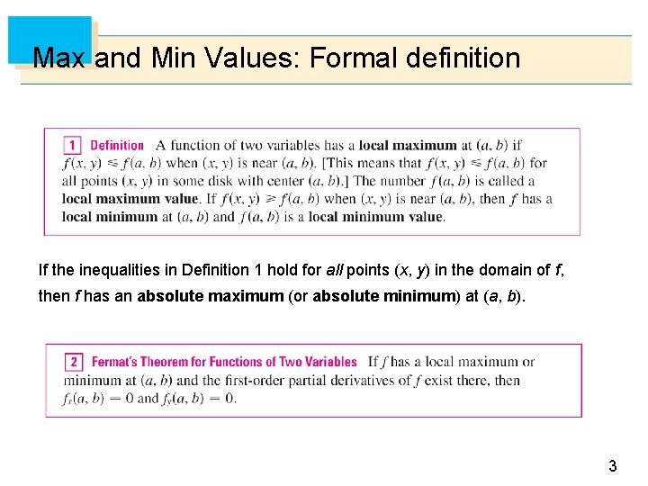
Max and Min Values: Formal definition If the inequalities in Definition 1 hold for all points (x, y) in the domain of f, then f has an absolute maximum (or absolute minimum) at (a, b). 3

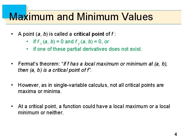
Maximum and Minimum Values • A point (a, b) is called a critical point of f : • if f x (a, b) = 0 and f y (a, b) = 0, or • if one of these partial derivatives does not exist. • Fermat’s theorem: “if f has a local maximum or minimum at (a, b), then (a, b) is a critical point of f”. • However, as in single-variable calculus, not all critical points are maxima or minima. • At a critical point, a function could have a local maximum or a local minimum or neither. 4

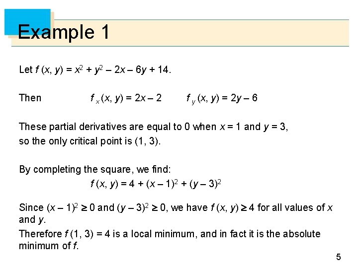
Example 1 Let f (x, y) = x 2 + y 2 – 2 x – 6 y + 14. Then f x (x, y) = 2 x – 2 f y (x, y) = 2 y – 6 These partial derivatives are equal to 0 when x = 1 and y = 3, so the only critical point is (1, 3). By completing the square, we find: f (x, y) = 4 + (x – 1)2 + (y – 3)2 Since (x – 1)2 0 and (y – 3)2 0, we have f (x, y) 4 for all values of x and y. Therefore f (1, 3) = 4 is a local minimum, and in fact it is the absolute minimum of f. 5

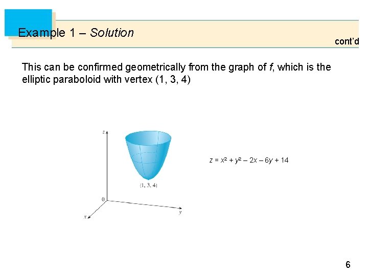
Example 1 – Solution cont’d This can be confirmed geometrically from the graph of f, which is the elliptic paraboloid with vertex (1, 3, 4) z = x 2 + y 2 – 2 x – 6 y + 14 6

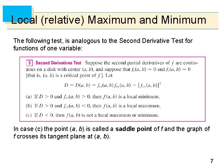
Local (relative) Maximum and Minimum The following test, is analogous to the Second Derivative Test for functions of one variable: In case (c) the point (a, b) is called a saddle point of f and the graph of f crosses its tangent plane at (a, b). 7

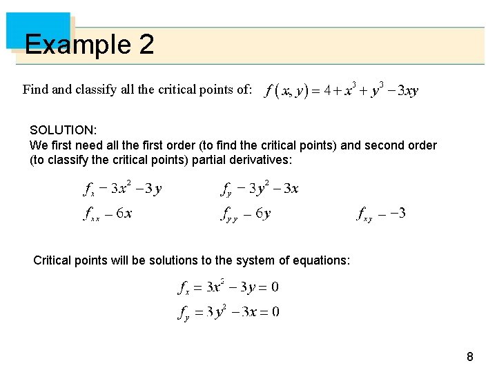
Example 2 Find and classify all the critical points of: . SOLUTION: We first need all the first order (to find the critical points) and second order (to classify the critical points) partial derivatives: Critical points will be solutions to the system of equations: 8

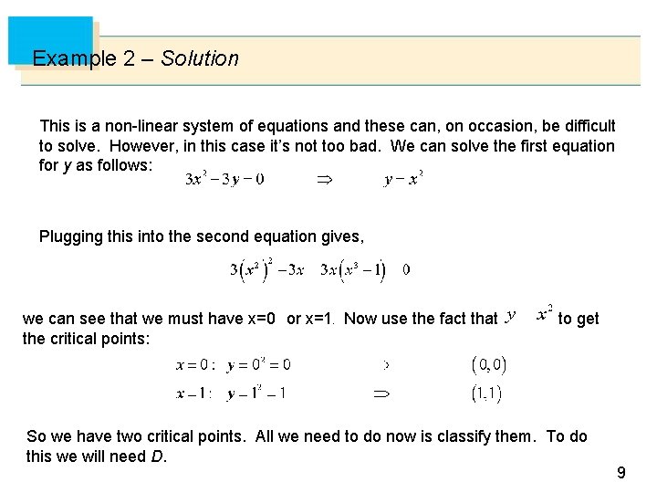
Example 2 – Solution This is a non-linear system of equations and these can, on occasion, be difficult to solve. However, in this case it’s not too bad. We can solve the first equation for y as follows: Plugging this into the second equation gives, we can see that we must have x=0 or x=1. Now use the fact that the critical points: to get So we have two critical points. All we need to do now is classify them. To do this we will need D. 9

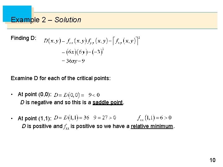
Example 2 – Solution Finding D: Examine D for each of the critical points: • At point (0, 0): D is negative and so this is a saddle point. • At point (1, 1): D is positive and fxx is positive so we have a relative minimum. 10

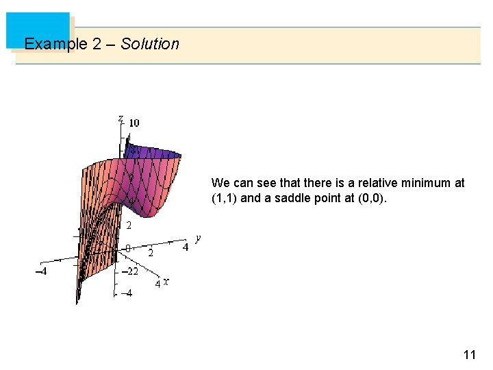
Example 2 – Solution We can see that there is a relative minimum at (1, 1) and a saddle point at (0, 0). 11

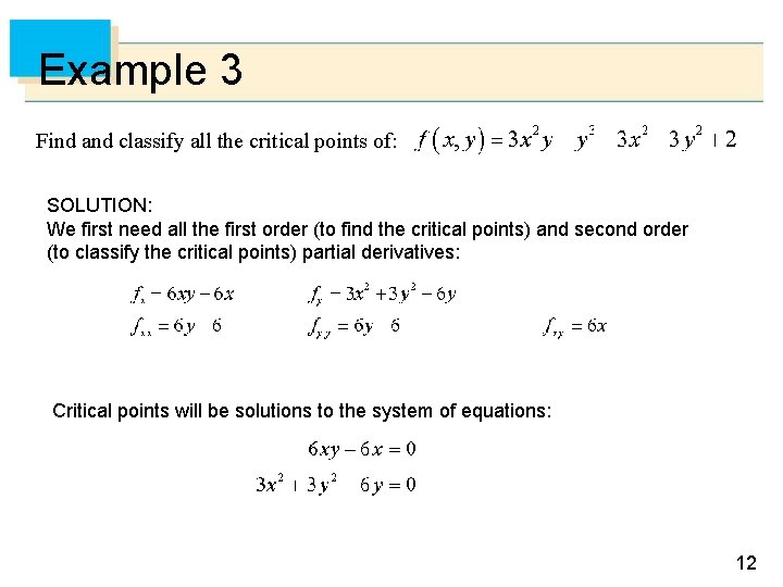
Example 3 Find and classify all the critical points of: SOLUTION: We first need all the first order (to find the critical points) and second order (to classify the critical points) partial derivatives: Critical points will be solutions to the system of equations: 12

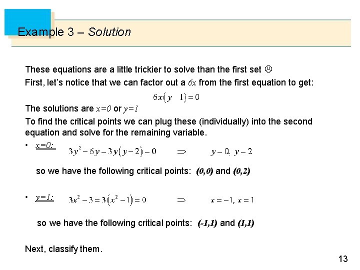
Example 3 – Solution These equations are a little trickier to solve than the first set First, let’s notice that we can factor out a 6 x from the first equation to get: The solutions are x=0 or y=1 To find the critical points we can plug these (individually) into the second equation and solve for the remaining variable. • x=0: so we have the following critical points: (0, 0) and (0, 2) • y=1: so we have the following critical points: (-1, 1) and (1, 1) Next, classify them. 13

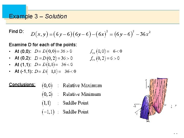
Example 3 – Solution Find D: Examine D for each of the points: • At (0, 0): • At (0, 2): • At (1, 1): • At (-1, 1): Conclusions: 14

Absolute Maximum and Minimum Values 15

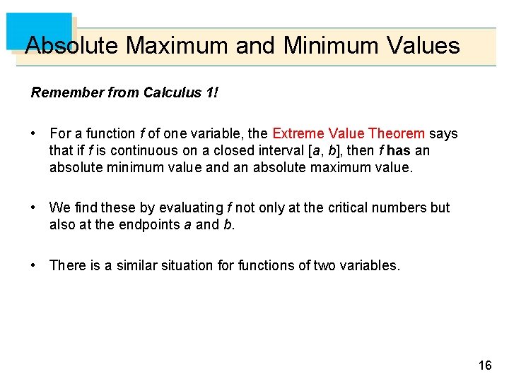
Absolute Maximum and Minimum Values Remember from Calculus 1! • For a function f of one variable, the Extreme Value Theorem says that if f is continuous on a closed interval [a, b], then f has an absolute minimum value and an absolute maximum value. • We find these by evaluating f not only at the critical numbers but also at the endpoints a and b. • There is a similar situation for functions of two variables. 16

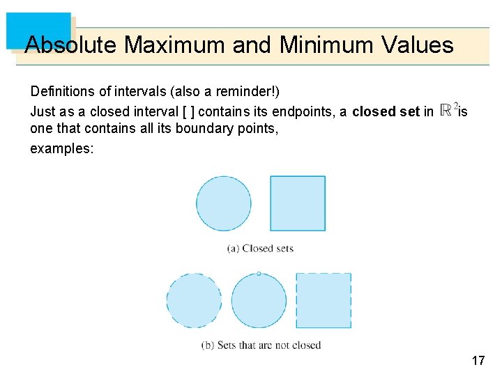
Absolute Maximum and Minimum Values Definitions of intervals (also a reminder!) Just as a closed interval [ ] contains its endpoints, a closed set in one that contains all its boundary points, examples: is 17

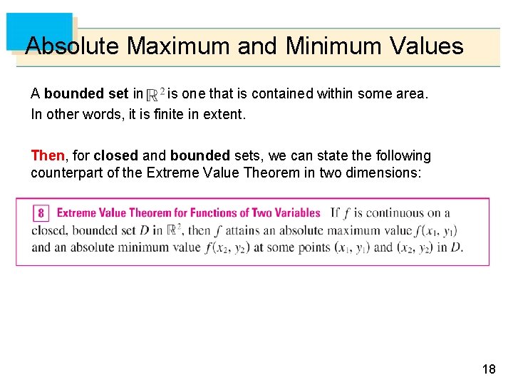
Absolute Maximum and Minimum Values A bounded set in is one that is contained within some area. In other words, it is finite in extent. Then, for closed and bounded sets, we can state the following counterpart of the Extreme Value Theorem in two dimensions: 18

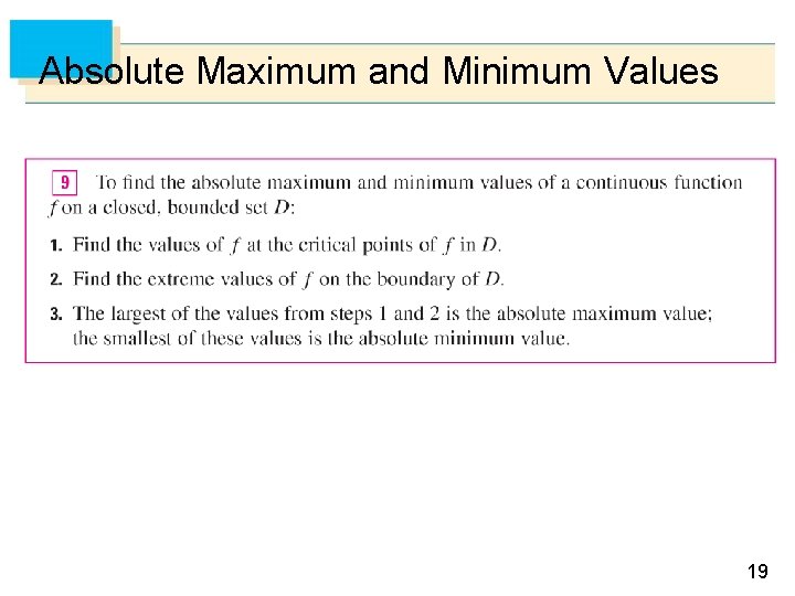
Absolute Maximum and Minimum Values 19

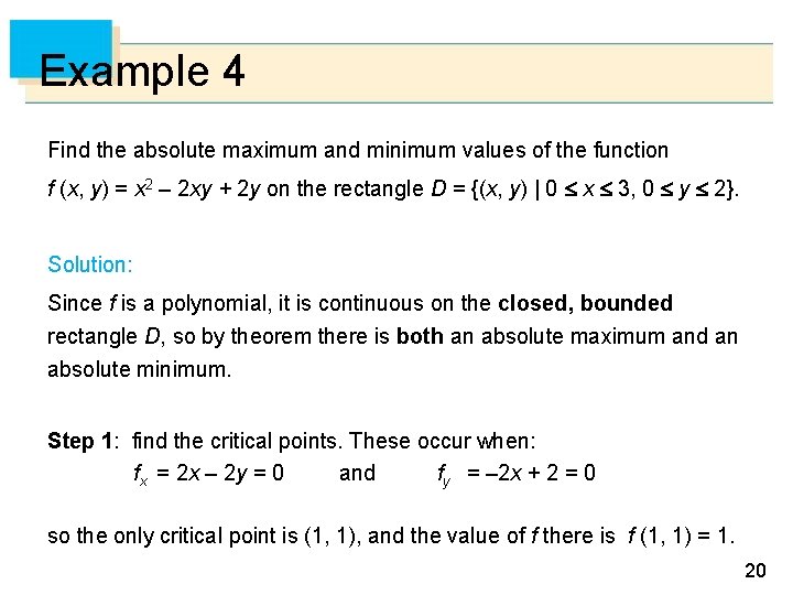
Example 4 Find the absolute maximum and minimum values of the function f (x, y) = x 2 – 2 xy + 2 y on the rectangle D = {(x, y) | 0 x 3, 0 y 2}. Solution: Since f is a polynomial, it is continuous on the closed, bounded rectangle D, so by theorem there is both an absolute maximum and an absolute minimum. Step 1: find the critical points. These occur when: fx = 2 x – 2 y = 0 and fy = – 2 x + 2 = 0 so the only critical point is (1, 1), and the value of f there is f (1, 1) = 1. 20

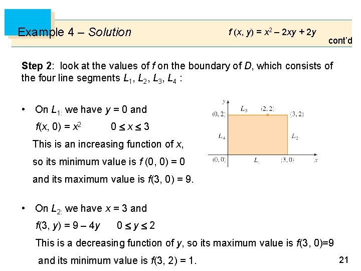
Example 4 – Solution f (x, y) = x 2 – 2 xy + 2 y cont’d Step 2: look at the values of f on the boundary of D, which consists of the four line segments L 1, L 2, L 3, L 4 : • On L 1: we have y = 0 and f(x, 0) = x 2 0 x 3 This is an increasing function of x, so its minimum value is f (0, 0) = 0 and its maximum value is f(3, 0) = 9. • On L 2: we have x = 3 and f(3, y) = 9 – 4 y 0 y 2 This is a decreasing function of y, so its maximum value is f(3, 0)=9 and its minimum value is f(3, 2) = 1. 21

Example 4 – Solution f(x, y) = x 2 – 2 xy + 2 y • On L 3: we have y = 2 and f(x, 2) = x 2 – 4 x + 4 cont’d 0 x 3 Simply by observing that f(x, 2) = (x – 2)2, we see that the minimum value of this function is f(2, 2) = 0 and the maximum value is f(0, 2) = 4. • Finally, on L 4 we have x = 0 and f(0, y) = 2 y 0 y 2 with maximum value f(0, 2) = 4 and minimum value f(0, 0) = 0. So on the boundary (all four sides), the minimum value of f is 0 and the maximum is 9. 22

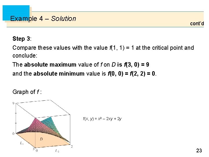
Example 4 – Solution cont’d Step 3: Compare these values with the value f(1, 1) = 1 at the critical point and conclude: The absolute maximum value of f on D is f(3, 0) = 9 and the absolute minimum value is f(0, 0) = f(2, 2) = 0. Graph of f : f (x, y) = x 2 – 2 xy + 2 y 23