14 1 CHAPTER 14 Capital Structure Decisions Part

14 - 1 CHAPTER 14 Capital Structure Decisions: Part I n Impact of leverage on returns n Business versus financial risk n Capital structure theory n Perpetual cash flow example n Setting the optimal capital structure in practice Copyright © 2002 South-Western

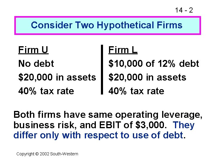
14 - 2 Consider Two Hypothetical Firms Firm U No debt $20, 000 in assets 40% tax rate Firm L $10, 000 of 12% debt $20, 000 in assets 40% tax rate Both firms have same operating leverage, business risk, and EBIT of $3, 000. They differ only with respect to use of debt. Copyright © 2002 South-Western

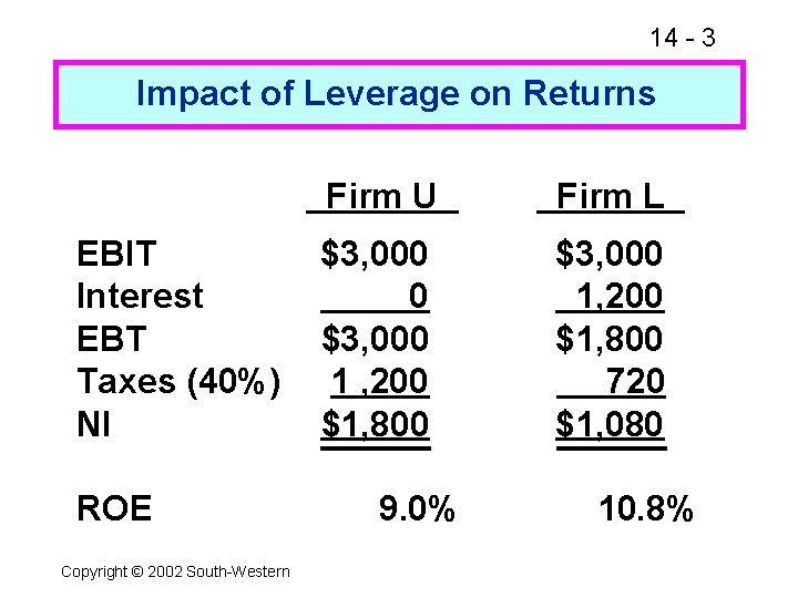
14 - 3 Impact of Leverage on Returns EBIT Interest EBT Taxes (40%) NI ROE Copyright © 2002 South-Western Firm U Firm L $3, 000 0 $3, 000 1 , 200 $1, 800 $3, 000 1, 200 $1, 800 720 $1, 080 9. 0% 10. 8%

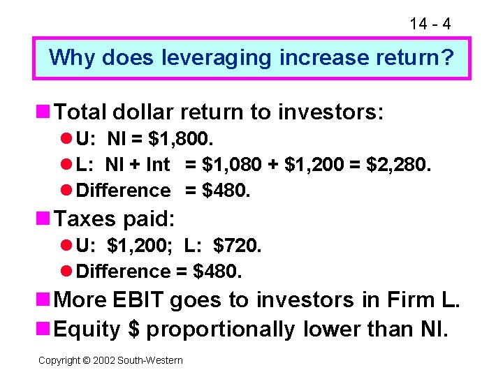
14 - 4 Why does leveraging increase return? n Total dollar return to investors: l U: NI = $1, 800. l L: NI + Int = $1, 080 + $1, 200 = $2, 280. l Difference = $480. n Taxes paid: l U: $1, 200; L: $720. l Difference = $480. n More EBIT goes to investors in Firm L. n Equity $ proportionally lower than NI. Copyright © 2002 South-Western

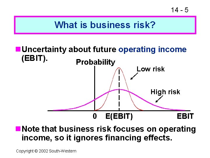
14 - 5 What is business risk? n. Uncertainty about future operating income (EBIT). Probability Low risk High risk 0 E(EBIT) EBIT n. Note that business risk focuses on operating income, so it ignores financing effects. Copyright © 2002 South-Western

14 - 6 Factors That Influence Business Risk n Uncertainty about demand (unit sales). n Uncertainty about output prices. n Uncertainty about input costs. n Product and other types of liability. n Degree of operating leverage (DOL). Copyright © 2002 South-Western

14 - 7 What is operating leverage, and how does it affect a firm’s business risk? n Operating leverage is the use of fixed costs rather than variable costs. n The higher the proportion of fixed costs within a firm’s overall cost structure, the greater the operating leverage. (More. . . ) Copyright © 2002 South-Western

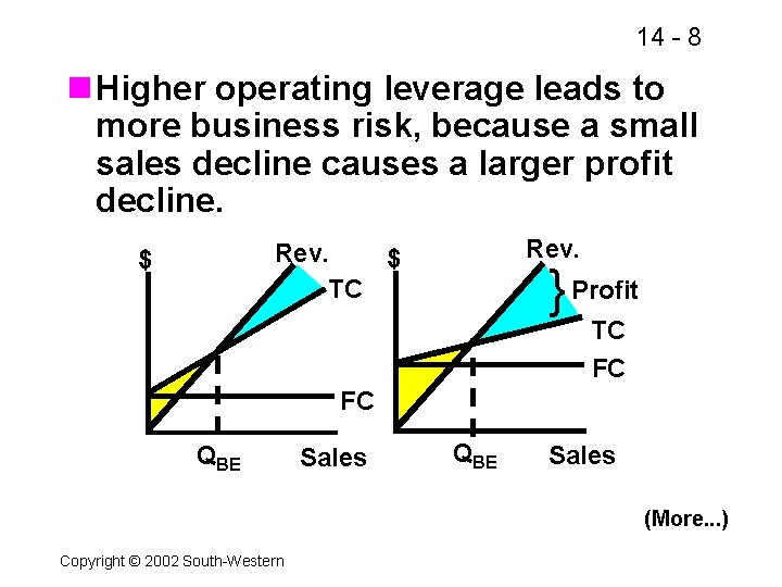
14 - 8 n Higher operating leverage leads to more business risk, because a small sales decline causes a larger profit decline. Rev. $ TC $ } Profit TC FC FC QBE Sales (More. . . ) Copyright © 2002 South-Western

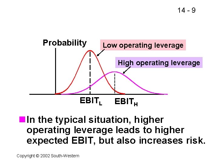
14 - 9 Probability Low operating leverage High operating leverage EBITL EBITH n In the typical situation, higher operating leverage leads to higher expected EBIT, but also increases risk. Copyright © 2002 South-Western

14 - 10 Business Risk versus Financial Risk n Business risk: l Uncertainty in future EBIT. l Depends on business factors such as competition, operating leverage, etc. n Financial risk: l Additional business risk concentrated on common stockholders when financial leverage is used. l Depends on the amount of debt and preferred stock financing. Copyright © 2002 South-Western

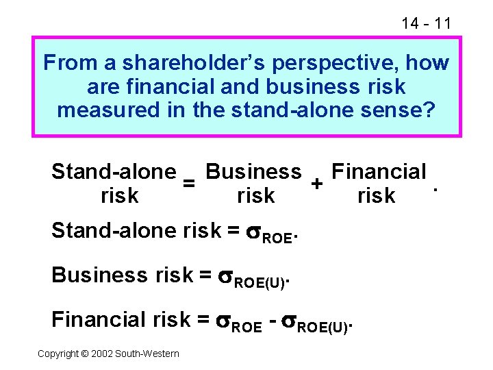
14 - 11 From a shareholder’s perspective, how are financial and business risk measured in the stand-alone sense? Stand-alone Business Financial = +. risk Stand-alone risk = ROE. Business risk = ROE(U). Financial risk = ROE - ROE(U). Copyright © 2002 South-Western

14 - 12 Now consider the fact that EBIT is not known with certainty. What is the impact of uncertainty on stockholder profitability and risk for Firm U and Firm L? Copyright © 2002 South-Western

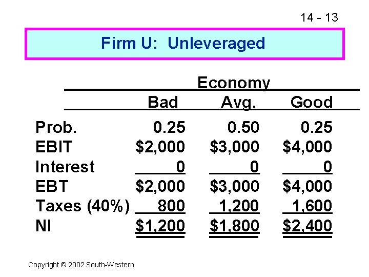
14 - 13 Firm U: Unleveraged Bad Prob. 0. 25 EBIT $2, 000 Interest 0 EBT $2, 000 Taxes (40%) 800 NI $1, 200 Copyright © 2002 South-Western Economy Avg. Good 0. 50 $3, 000 1, 200 $1, 800 0. 25 $4, 000 0 $4, 000 1, 600 $2, 400

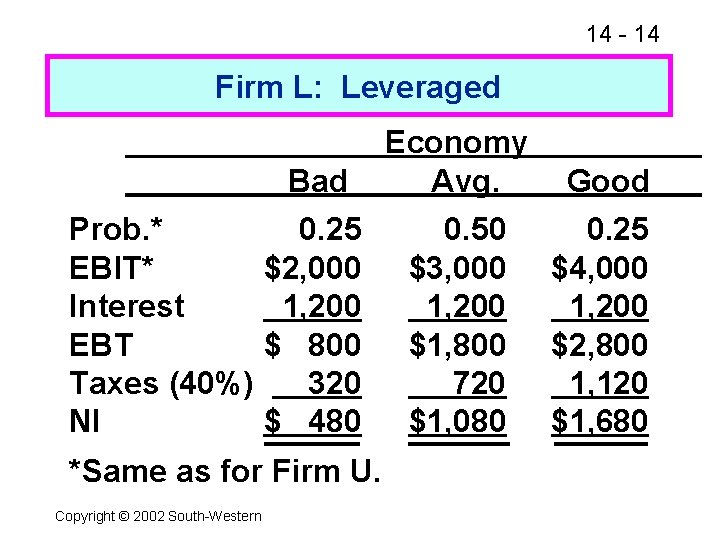
14 - 14 Firm L: Leveraged Prob. * EBIT* Interest EBT Taxes (40%) NI Bad Economy Avg. Good 0. 25 $2, 000 1, 200 $ 800 320 $ 480 0. 50 $3, 000 1, 200 $1, 800 720 $1, 080 0. 25 $4, 000 1, 200 $2, 800 1, 120 $1, 680 *Same as for Firm U. Copyright © 2002 South-Western

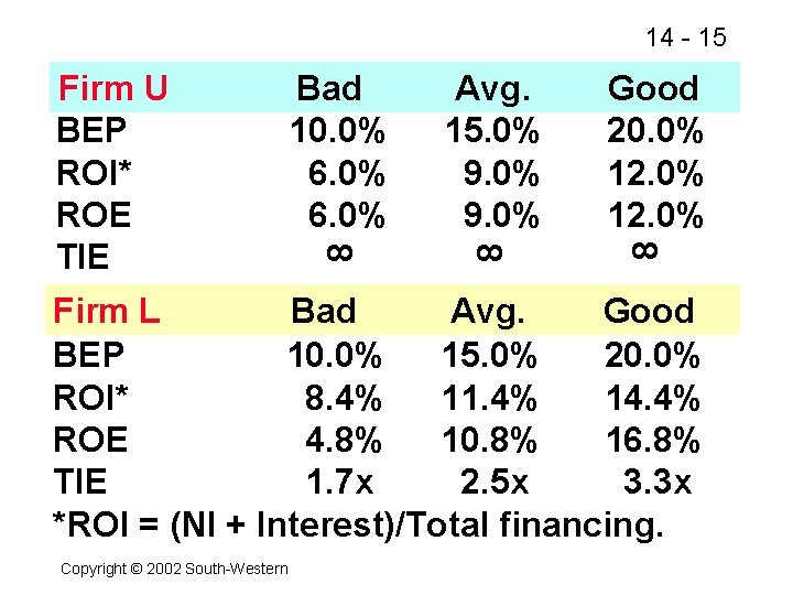
Avg. 15. 0% 9. 0% Good 20. 0% 12. 0% 8 Bad 10. 0% 6. 0% 8 Firm U BEP ROI* ROE TIE 8 14 - 15 Firm L Bad Avg. Good BEP 10. 0% 15. 0% 20. 0% ROI* 8. 4% 11. 4% 14. 4% ROE 4. 8% 10. 8% 16. 8% TIE 1. 7 x 2. 5 x 3. 3 x *ROI = (NI + Interest)/Total financing. Copyright © 2002 South-Western

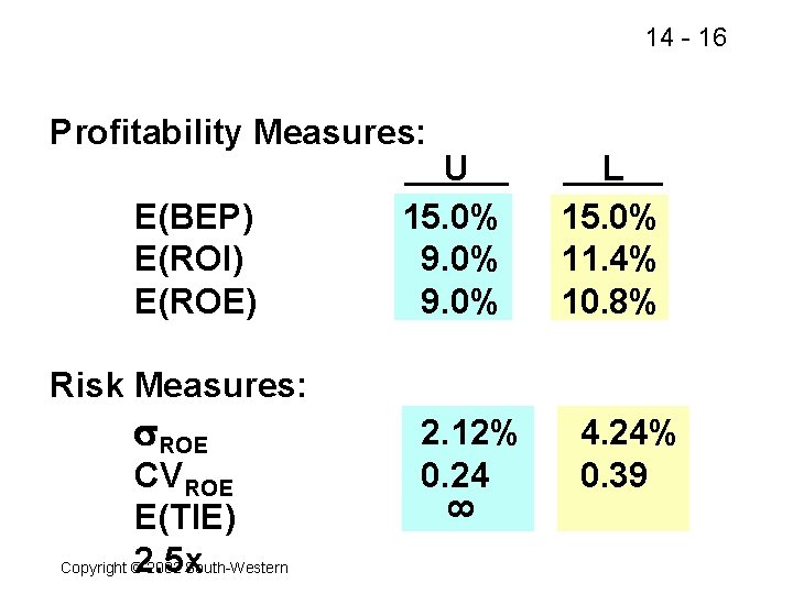
14 - 16 Profitability Measures: E(BEP) E(ROI) E(ROE) U 15. 0% 9. 0% L 15. 0% 11. 4% 10. 8% Risk Measures: CVROE E(TIE) 2. 5 x Copyright © 2002 South-Western 2. 12% 0. 24 8 ROE 4. 24% 0. 39

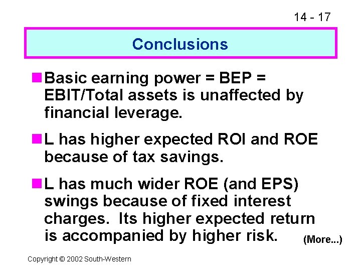
14 - 17 Conclusions n Basic earning power = BEP = EBIT/Total assets is unaffected by financial leverage. n L has higher expected ROI and ROE because of tax savings. n L has much wider ROE (and EPS) swings because of fixed interest charges. Its higher expected return is accompanied by higher risk. (More. . . ) Copyright © 2002 South-Western

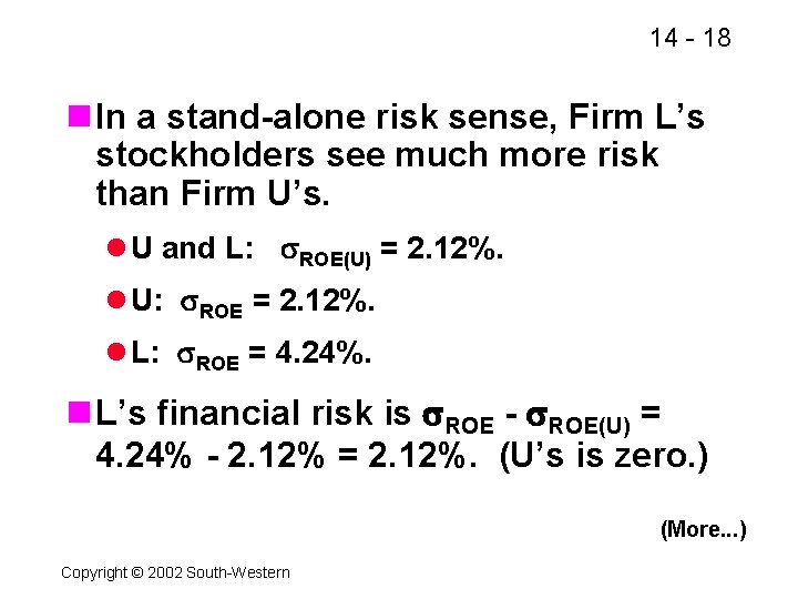
14 - 18 n In a stand-alone risk sense, Firm L’s stockholders see much more risk than Firm U’s. l U and L: ROE(U) = 2. 12%. l U: ROE = 2. 12%. l L: ROE = 4. 24%. n L’s financial risk is ROE - ROE(U) = 4. 24% - 2. 12% = 2. 12%. (U’s is zero. ) (More. . . ) Copyright © 2002 South-Western

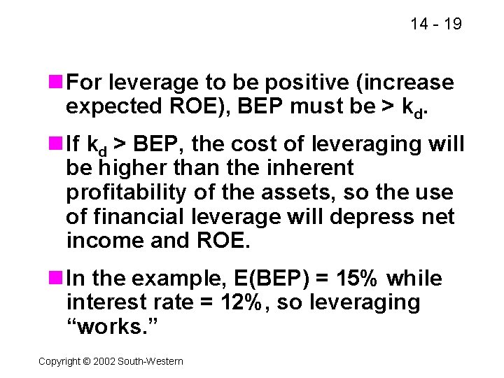
14 - 19 n For leverage to be positive (increase expected ROE), BEP must be > kd. n If kd > BEP, the cost of leveraging will be higher than the inherent profitability of the assets, so the use of financial leverage will depress net income and ROE. n In the example, E(BEP) = 15% while interest rate = 12%, so leveraging “works. ” Copyright © 2002 South-Western

14 - 20 Capital Structure Theory n MM theory l Zero taxes l Corporate and personal taxes n Trade-off theory n Signaling theory n Debt financing as a managerial constraint Copyright © 2002 South-Western

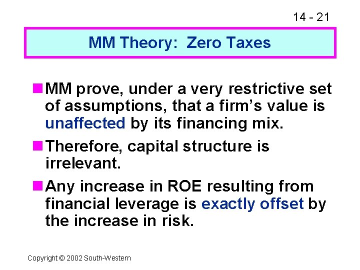
14 - 21 MM Theory: Zero Taxes n MM prove, under a very restrictive set of assumptions, that a firm’s value is unaffected by its financing mix. n Therefore, capital structure is irrelevant. n Any increase in ROE resulting from financial leverage is exactly offset by the increase in risk. Copyright © 2002 South-Western

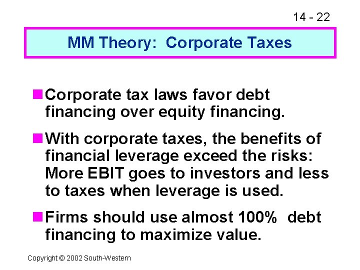
14 - 22 MM Theory: Corporate Taxes n Corporate tax laws favor debt financing over equity financing. n With corporate taxes, the benefits of financial leverage exceed the risks: More EBIT goes to investors and less to taxes when leverage is used. n Firms should use almost 100% debt financing to maximize value. Copyright © 2002 South-Western

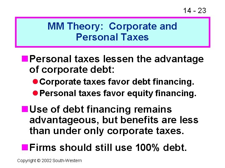
14 - 23 MM Theory: Corporate and Personal Taxes n Personal taxes lessen the advantage of corporate debt: l Corporate taxes favor debt financing. l Personal taxes favor equity financing. n Use of debt financing remains advantageous, but benefits are less than under only corporate taxes. n Firms should still use 100% debt. Copyright © 2002 South-Western

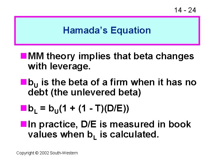
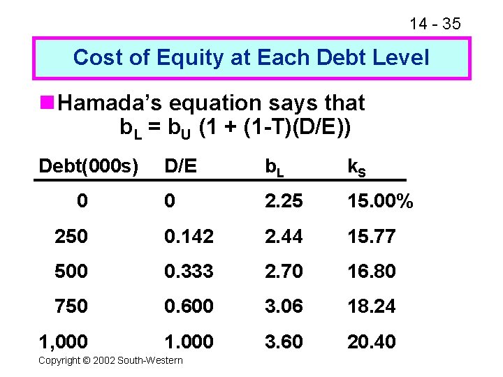
14 - 24 Hamada’s Equation n MM theory implies that beta changes with leverage. n b. U is the beta of a firm when it has no debt (the unlevered beta) n b. L = b. U(1 + (1 - T)(D/E)) n In practice, D/E is measured in book values when b. L is calculated. Copyright © 2002 South-Western

14 - 25 Trade-off Theory n MM theory ignores bankruptcy (financial distress) costs, which increase as more leverage is used. n At low leverage levels, tax benefits outweigh bankruptcy costs. n At high levels, bankruptcy costs outweigh tax benefits. n An optimal capital structure exists that balances these costs and benefits. Copyright © 2002 South-Western

14 - 26 Signaling Theory n MM assumed that investors and managers have the same information. n But, managers often have better information. Thus, they would: l Sell stock if stock is overvalued. l Sell bonds if stock is undervalued. n Investors understand this, so view new stock sales as a negative signal. n Implications for managers? Copyright © 2002 South-Western

14 - 27 Debt Financing As a Managerial Constraint n One agency problem is that managers can use corporate funds for non-value maximizing purposes. n The use of financial leverage: l Bonds “free cash flow. ” l Forces discipline on managers. n However, it also increases risk of financial distress. Copyright © 2002 South-Western

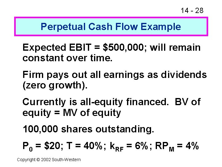
14 - 28 Perpetual Cash Flow Example Expected EBIT = $500, 000; will remain constant over time. Firm pays out all earnings as dividends (zero growth). Currently is all-equity financed. BV of equity = MV of equity 100, 000 shares outstanding. P 0 = $20; T = 40%; k. RF = 6%; RPM = 4% Copyright © 2002 South-Western

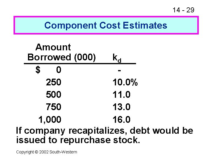
14 - 29 Component Cost Estimates Amount Borrowed (000) kd $ 0 250 10. 0% 500 11. 0 750 13. 0 1, 000 16. 0 If company recapitalizes, debt would be issued to repurchase stock. Copyright © 2002 South-Western

14 - 30 n The MM and Miller models cannot be applied directly because several assumptions are violated. lkd is not a constant. l. Bankruptcy and agency costs exist. n In practice, Hamada’s equation is used to find k. S for the firm with different levels of debt. Copyright © 2002 South-Western

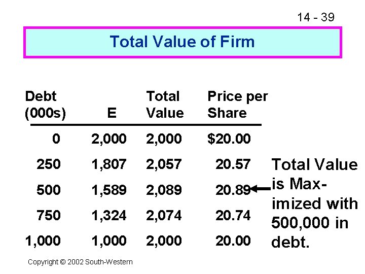
14 - 31 The Optimal Capital Structure n Calculate the cost of equity at each level of debt. n Calculate the value of equity at each level of debt. n Calculate the total value of the firm (value of equity + value of debt) at each level of debt. n The optimal capital structure maximizes the total value of the firm. Copyright © 2002 South-Western

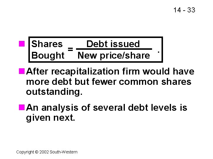
14 - 32 Sequence of Events in a Recapitalization n Firm announces the recapitalization. n Investors reassess their views and estimate a new equity value. n New debt is issued and proceeds are used to repurchase stock at the new equilibrium price. (More. . . ) Copyright © 2002 South-Western

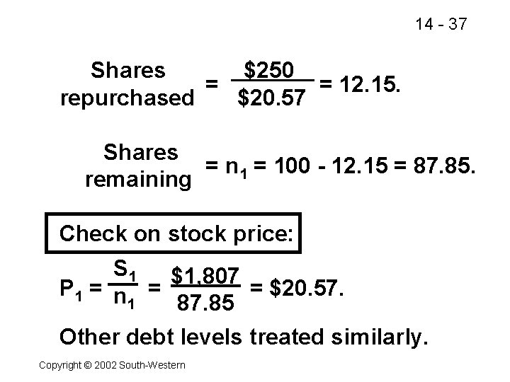
14 - 33 n Shares Debt issued =. Bought New price/share n After recapitalization firm would have more debt but fewer common shares outstanding. n An analysis of several debt levels is given next. Copyright © 2002 South-Western

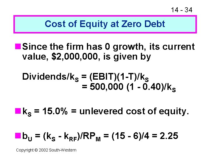
14 - 34 Cost of Equity at Zero Debt n Since the firm has 0 growth, its current value, $2, 000, is given by Dividends/k. S = (EBIT)(1 -T)/k. S = 500, 000 (1 - 0. 40)/k. S n k. S = 15. 0% = unlevered cost of equity. n b. U = (k. S - k. RF)/RPM = (15 - 6)/4 = 2. 25 Copyright © 2002 South-Western

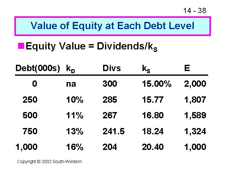
14 - 35 Cost of Equity at Each Debt Level n Hamada’s equation says that b. L = b. U (1 + (1 -T)(D/E)) Debt(000 s) D/E b. L k. S 0 2. 25 15. 00% 250 0. 142 2. 44 15. 77 500 0. 333 2. 70 16. 80 750 0. 600 3. 06 18. 24 1, 000 1. 000 3. 60 20. 40 0 Copyright © 2002 South-Western

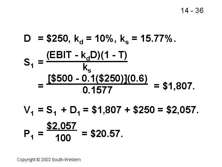
14 - 36 D = $250, kd = 10%, ks = 15. 77%. (EBIT - kd. D)(1 - T) S 1 = ks [$500 - 0. 1($250)](0. 6) = = $1, 807. 0. 1577 V 1 = S 1 + D 1 = $1, 807 + $250 = $2, 057 P 1 = 100 = $20. 57. Copyright © 2002 South-Western

14 - 37 Shares $250 = = 12. 15. repurchased $20. 57 Shares = n 1 = 100 - 12. 15 = 87. 85. remaining Check on stock price: S 1 $1, 807 P 1 = n = = $20. 57. 1 87. 85 Other debt levels treated similarly. Copyright © 2002 South-Western

14 - 38 Value of Equity at Each Debt Level n Equity Value = Dividends/k. S Debt(000 s) k. D Divs k. S E na 300 15. 00% 2, 000 250 10% 285 15. 77 1, 807 500 11% 267 16. 80 1, 589 750 13% 241. 5 18. 24 1, 324 1, 000 16% 204 20. 40 1, 000 0 Copyright © 2002 South-Western

14 - 39 Total Value of Firm Debt (000 s) E Total Value Price per Share 0 2, 000 $20. 00 250 1, 807 2, 057 20. 57 500 1, 589 2, 089 20. 89 750 1, 324 2, 074 20. 74 1, 000 2, 000 20. 00 Copyright © 2002 South-Western Total Value is Maximized with 500, 000 in debt.

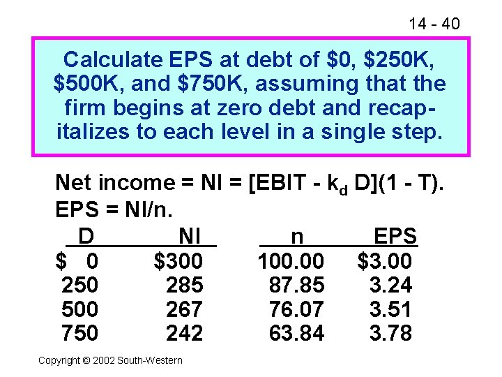
14 - 40 Calculate EPS at debt of $0, $250 K, $500 K, and $750 K, assuming that the firm begins at zero debt and recapitalizes to each level in a single step. Net income = NI = [EBIT - kd D](1 - T). EPS = NI/n. D NI n EPS $ 0 $300 100. 00 $3. 00 250 285 87. 85 3. 24 500 267 76. 07 3. 51 750 242 63. 84 3. 78 Copyright © 2002 South-Western

14 - 41 n EPS continues to increase beyond the $500, 000 optimal debt level. n Does this mean that the optimal debt level is $750, 000, or even higher? Copyright © 2002 South-Western

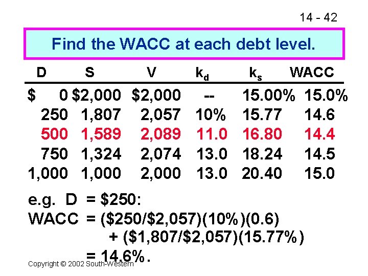
14 - 42 Find the WACC at each debt level. D $ S V kd ks WACC 0 $2, 000 -15. 00% 250 1, 807 2, 057 10% 15. 77 500 1, 589 2, 089 11. 0 16. 80 750 1, 324 2, 074 13. 0 18. 24 1, 000 2, 000 13. 0 20. 40 15. 0% 14. 6 14. 4 14. 5 15. 0 e. g. D = $250: WACC = ($250/$2, 057)(10%)(0. 6) + ($1, 807/$2, 057)(15. 77%) = 14. 6%. Copyright © 2002 South-Western

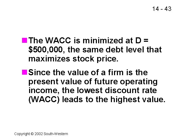
14 - 43 n The WACC is minimized at D = $500, 000, the same debt level that maximizes stock price. n Since the value of a firm is the present value of future operating income, the lowest discount rate (WACC) leads to the highest value. Copyright © 2002 South-Western

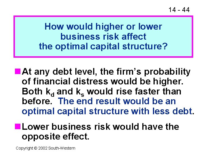
14 - 44 How would higher or lower business risk affect the optimal capital structure? n At any debt level, the firm’s probability of financial distress would be higher. Both kd and ks would rise faster than before. The end result would be an optimal capital structure with less debt. n Lower business risk would have the opposite effect. Copyright © 2002 South-Western

14 - 45 Is it possible to do an analysis exactly like the one above for most firms? n No. The analysis above was based on the assumption of zero growth, and most firms do not fit this category. n Further, it would be very difficult, if not impossible, to estimate ks with any confidence. Copyright © 2002 South-Western

14 - 46 What type of analysis should firms conduct to help find their optimal, or target, capital structure? n Financial forecasting models can help show capital structure changes are likely to affect stock prices, coverage ratios, and so on. (More. . . ) Copyright © 2002 South-Western

14 - 47 n Forecasting models can generate results under various scenarios, but the financial manager must specify appropriate input values, interpret the output, and eventually decide on a target capital structure. n In the end, capital structure decision will be based on a combination of analysis and judgment. Copyright © 2002 South-Western

14 - 48 What other factors would managers consider when setting the target capital structure? n Debt ratios of other firms in the industry. n Pro forma coverage ratios at different capital structures under different economic scenarios. n Lender and rating agency attitudes (impact on bond ratings). Copyright © 2002 South-Western

14 - 49 n Reserve borrowing capacity. n Effects on control. n Type of assets: Are they tangible, and hence suitable as collateral? n Tax rates. Copyright © 2002 South-Western