13 Functions of Several Variables Copyright Cengage Learning

13. 9 Applications of Extrema of Functions of Two Variables Copyright © Cengage Learning.

Objectives n Solve optimization problems involving functions of several variables. n Use the method of least squares. 3

Applied Optimization Problems 4

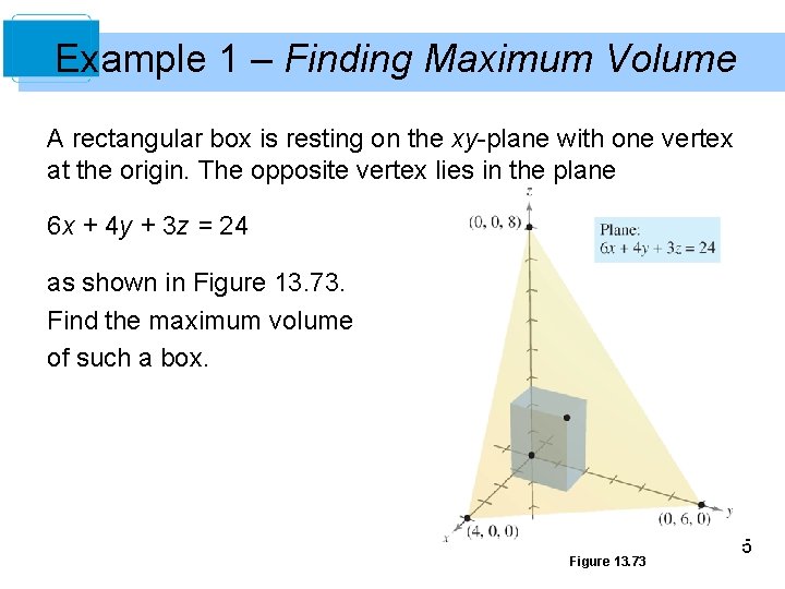
Example 1 – Finding Maximum Volume A rectangular box is resting on the xy-plane with one vertex at the origin. The opposite vertex lies in the plane 6 x + 4 y + 3 z = 24 as shown in Figure 13. 73. Find the maximum volume of such a box. Figure 13. 73 5

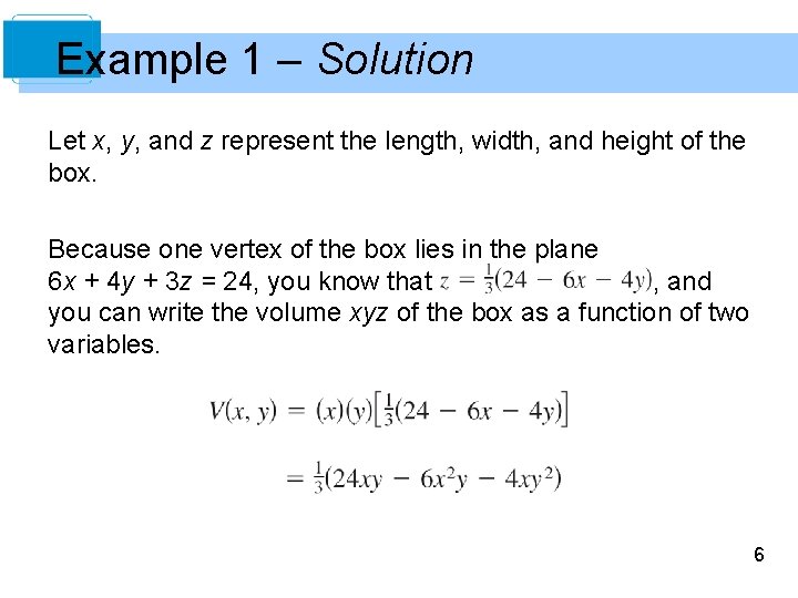
Example 1 – Solution Let x, y, and z represent the length, width, and height of the box. Because one vertex of the box lies in the plane 6 x + 4 y + 3 z = 24, you know that , and you can write the volume xyz of the box as a function of two variables. 6

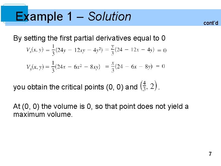
Example 1 – Solution cont’d By setting the first partial derivatives equal to 0 you obtain the critical points (0, 0) and . At (0, 0) the volume is 0, so that point does not yield a maximum volume. 7

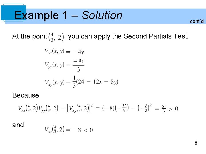
Example 1 – Solution At the point cont’d , you can apply the Second Partials Test. Because and 8

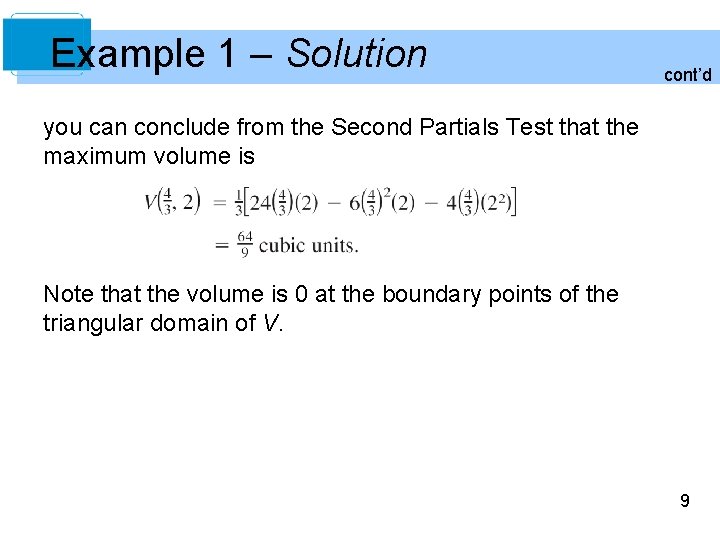
Example 1 – Solution cont’d you can conclude from the Second Partials Test that the maximum volume is Note that the volume is 0 at the boundary points of the triangular domain of V. 9

The Method of Least Squares 10

The Method of Least Squares Many examples involves mathematical models. For example, Example 2 in this section is about a quadratic model for profit. There are several ways to develop such models; one is called the method of least squares. In constructing a model to represent a particular phenomenon, the goals are simplicity and accuracy. Of course, these goals often conflict. 11

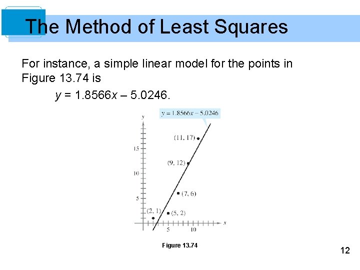
The Method of Least Squares For instance, a simple linear model for the points in Figure 13. 74 is y = 1. 8566 x – 5. 0246. Figure 13. 74 12

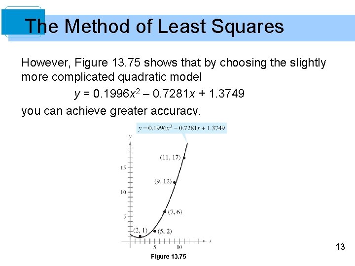
The Method of Least Squares However, Figure 13. 75 shows that by choosing the slightly more complicated quadratic model y = 0. 1996 x 2 – 0. 7281 x + 1. 3749 you can achieve greater accuracy. 13 Figure 13. 75

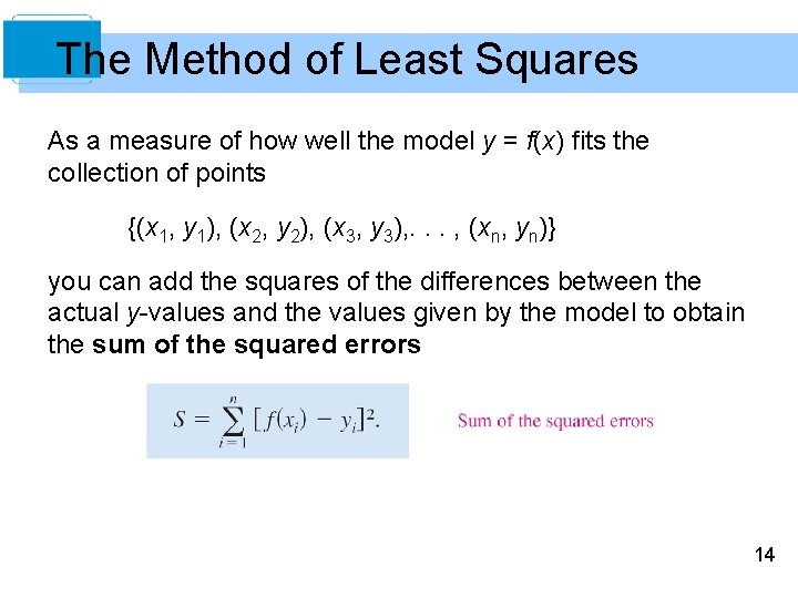
The Method of Least Squares As a measure of how well the model y = f(x) fits the collection of points {(x 1, y 1), (x 2, y 2), (x 3, y 3), . . . , (xn, yn)} you can add the squares of the differences between the actual y-values and the values given by the model to obtain the sum of the squared errors 14

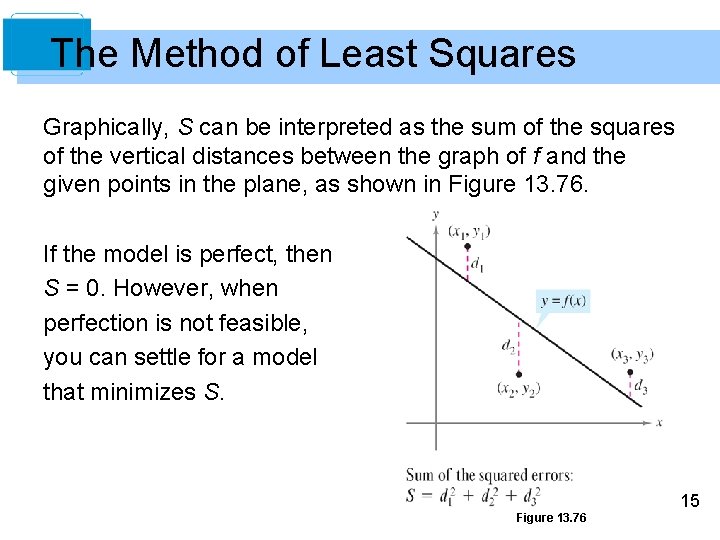
The Method of Least Squares Graphically, S can be interpreted as the sum of the squares of the vertical distances between the graph of f and the given points in the plane, as shown in Figure 13. 76. If the model is perfect, then S = 0. However, when perfection is not feasible, you can settle for a model that minimizes S. Figure 13. 76 15

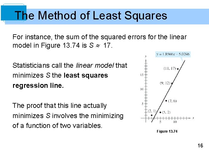
The Method of Least Squares For instance, the sum of the squared errors for the linear model in Figure 13. 74 is S 17. Statisticians call the linear model that minimizes S the least squares regression line. The proof that this line actually minimizes S involves the minimizing of a function of two variables. Figure 13. 74 16

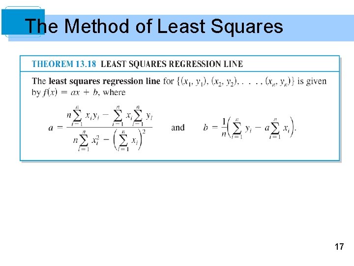
The Method of Least Squares 17

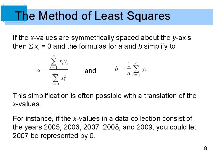
The Method of Least Squares If the x-values are symmetrically spaced about the y-axis, then xi = 0 and the formulas for a and b simplify to and This simplification is often possible with a translation of the x-values. For instance, if the x-values in a data collection consist of the years 2005, 2006, 2007, 2008, and 2009, you could let 2007 be represented by 0. 18

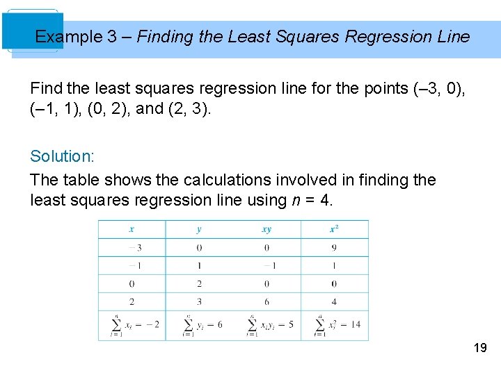
Example 3 – Finding the Least Squares Regression Line Find the least squares regression line for the points (– 3, 0), (– 1, 1), (0, 2), and (2, 3). Solution: The table shows the calculations involved in finding the least squares regression line using n = 4. 19

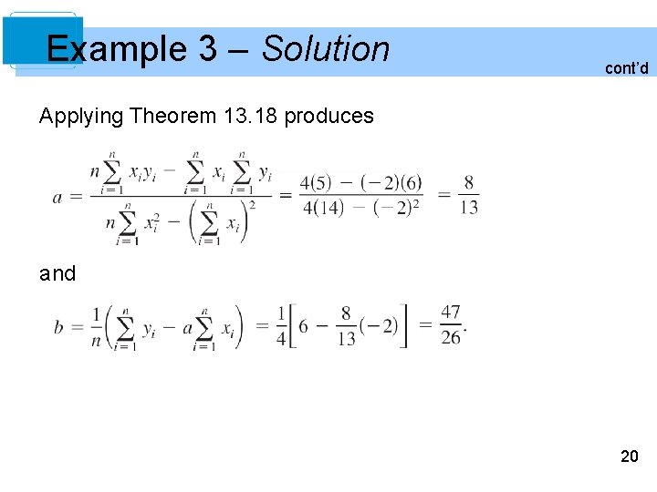
Example 3 – Solution cont’d Applying Theorem 13. 18 produces and 20

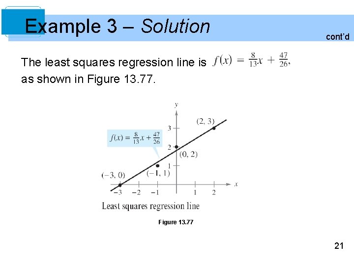
Example 3 – Solution cont’d The least squares regression line is as shown in Figure 13. 77 21