13 Functional Forms Examples of Choosing Functional Forms

13. Functional Forms ØExamples of Choosing Functional Forms ØInterpreting Econ Models ØThe Error Term 1

13. 1 Functional Forms To explain and predict the relationship between variables, it is ESSENTIAL to know the correct graph or functional form. The wrong functional form can lead to the wrong conclusion: 2

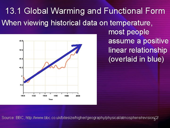
13. 1 Global Warming and Functional Form When viewing historical data on temperature, most people assume a positive linear relationship (overlaid in blue) Source: BBC, http: //www. bbc. co. uk/bitesize/higher/geography/physical/atmosphere/revision/2/ 3

13. 1 Global Warming and Functional Form In his 2006 film, “An Inconvenient Truth”, Al Gore advocated a more exponential relationship: 4 Source: An Inconvenient Truth (2016) screen shot. Blue trend line added

13. 1 Global Warming and Functional Form In laboratory settings, the pure greenhouse effect is seen to have a logarithmic relationship: 5 Source: Myhre et al (1988). Copied from http: //www. moralcaseforfossilfuels. com/data/

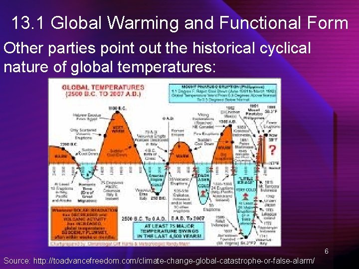
13. 1 Global Warming and Functional Form Other parties point out the historical cyclical nature of global temperatures: 6 Source: http: //toadvancefreedom. com/climate-change-global-catastrophe-or-false-alarm/

13. 1 Global Warming and Functional Form Different relationships between variables (different functional forms) can lead to different conclusions. THE FUNCTIONAL FORM MATTERS! 7

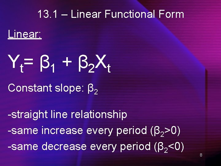
13. 1 – Linear Functional Form Linear: Y t = β 1 + β 2 X t Constant slope: β 2 -straight line relationship -same increase every period (β 2>0) -same decrease every period (β 2<0) 8

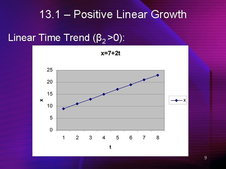
13. 1 – Positive Linear Growth Linear Time Trend (β 2 >0): 9

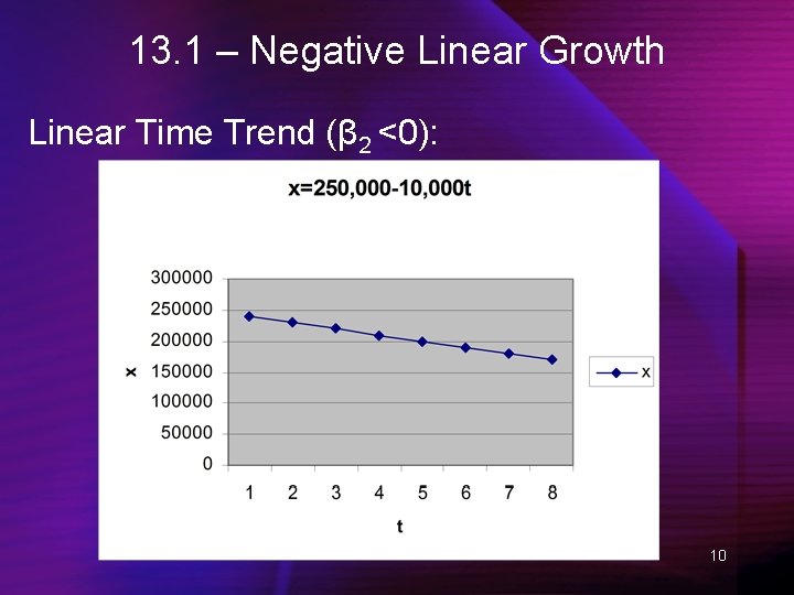
13. 1 – Negative Linear Growth Linear Time Trend (β 2 <0): 10

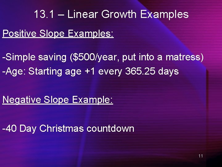
13. 1 – Linear Growth Examples Positive Slope Examples: -Simple saving ($500/year, put into a matress) -Age: Starting age +1 every 365. 25 days Negative Slope Example: -40 Day Christmas countdown 11

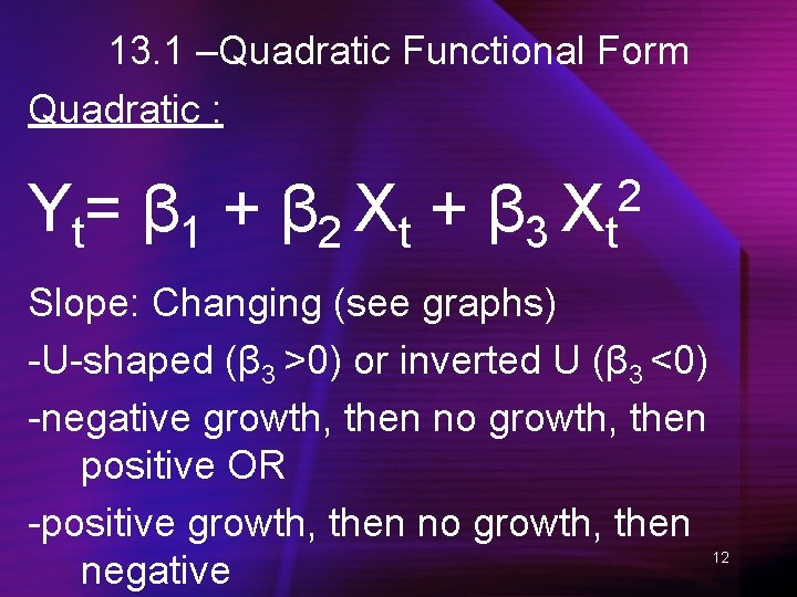
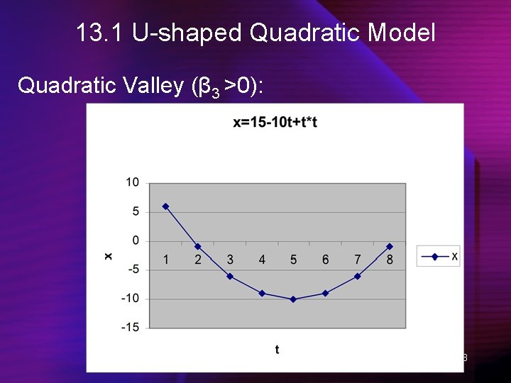
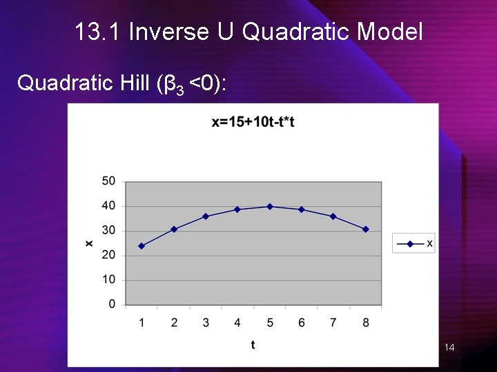
13. 1 –Quadratic Functional Form Quadratic : Y t = β 1 + β 2 X t + 2 β 3 Xt Slope: Changing (see graphs) -U-shaped (β 3 >0) or inverted U (β 3 <0) -negative growth, then no growth, then positive OR -positive growth, then no growth, then negative 12

13. 1 U-shaped Quadratic Model Quadratic Valley (β 3 >0): 13

13. 1 Inverse U Quadratic Model Quadratic Hill (β 3 <0): 14

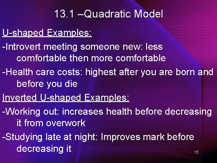
13. 1 –Quadratic Model U-shaped Examples: -Introvert meeting someone new: less comfortable then more comfortable -Health care costs: highest after you are born and before you die Inverted U-shaped Examples: -Working out: increases health before decreasing it from overwork -Studying late at night: Improves mark before decreasing it 15

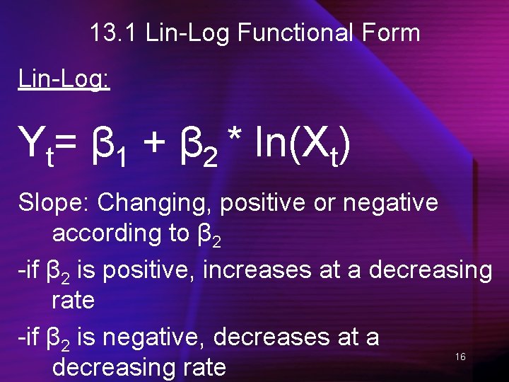
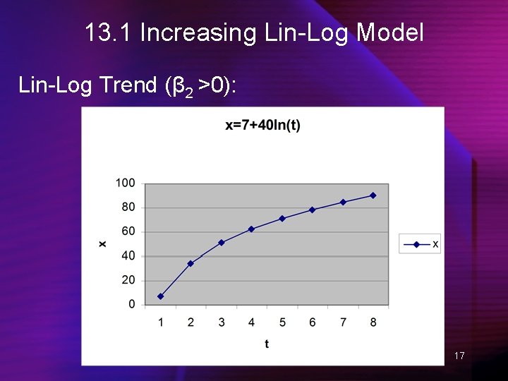
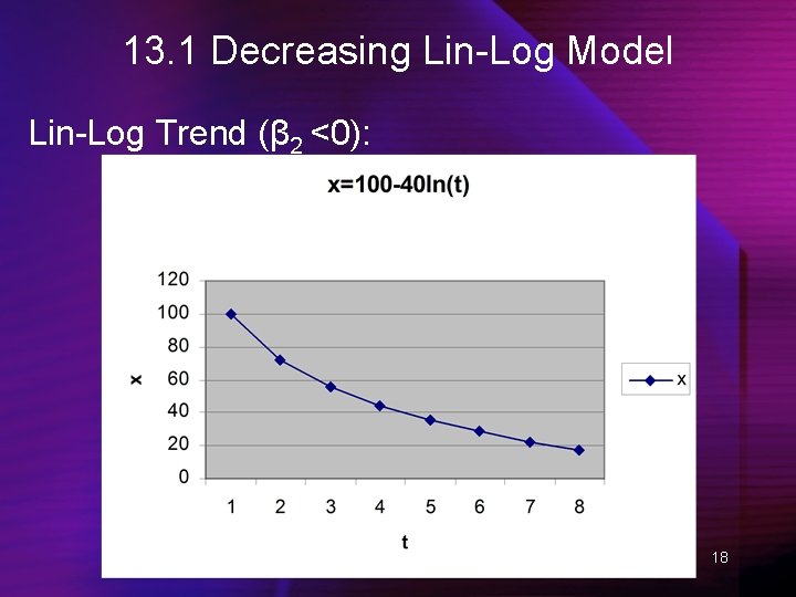
13. 1 Lin-Log Functional Form Lin-Log: Yt= β 1 + β 2 * ln(Xt) Slope: Changing, positive or negative according to β 2 -if β 2 is positive, increases at a decreasing rate -if β 2 is negative, decreases at a decreasing rate 16

13. 1 Increasing Lin-Log Model Lin-Log Trend (β 2 >0): 17

13. 1 Decreasing Lin-Log Model Lin-Log Trend (β 2 <0): 18

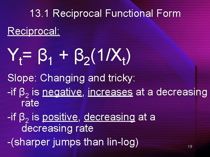
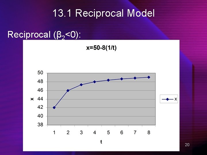
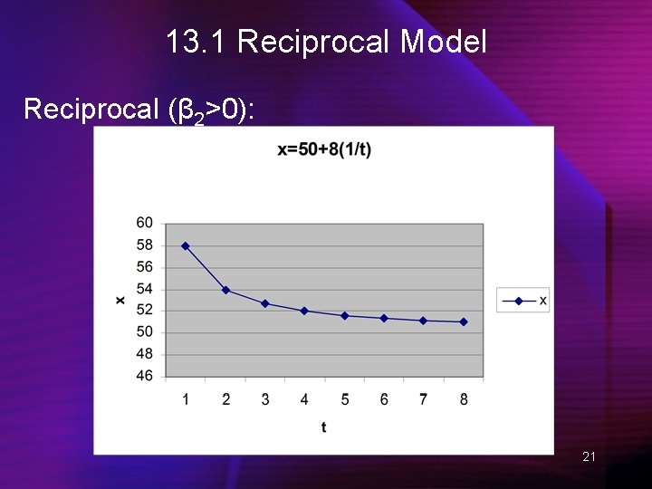
13. 1 Reciprocal Functional Form Reciprocal: Yt= β 1 + β 2(1/Xt) Slope: Changing and tricky: -if β 2 is negative, increases at a decreasing rate -if β 2 is positive, decreasing at a decreasing rate -(sharper jumps than lin-log) 19

13. 1 Reciprocal Model Reciprocal (β 2<0): 20

13. 1 Reciprocal Model Reciprocal (β 2>0): 21

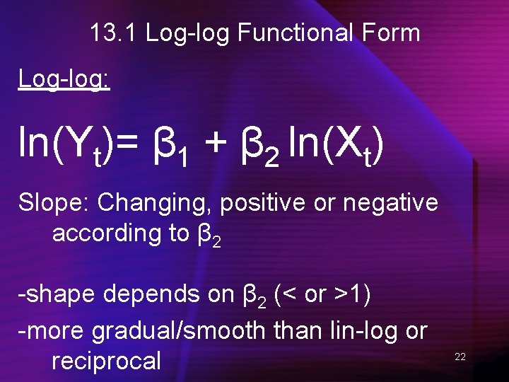
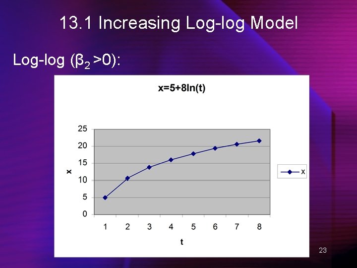
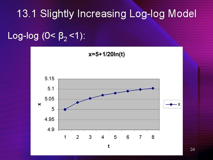
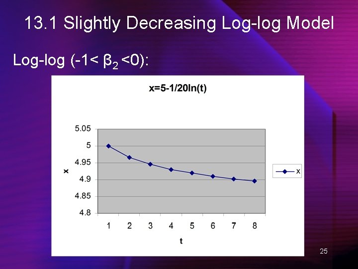
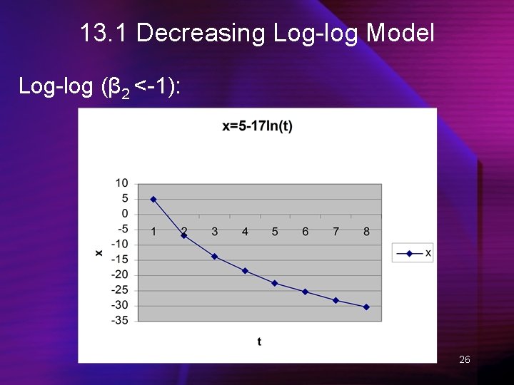
13. 1 Log-log Functional Form Log-log: ln(Yt)= β 1 + β 2 ln(Xt) Slope: Changing, positive or negative according to β 2 -shape depends on β 2 (< or >1) -more gradual/smooth than lin-log or reciprocal 22

13. 1 Increasing Log-log Model Log-log (β 2 >0): 23

13. 1 Slightly Increasing Log-log Model Log-log (0< β 2 <1): 24

13. 1 Slightly Decreasing Log-log Model Log-log (-1< β 2 <0): 25

13. 1 Decreasing Log-log Model Log-log (β 2 <-1): 26

13. 1 Positive Slope Model Examples: -Studying: each hour yields less as you approach perfect (diminishing marginal returns) -Pizza: Your enjoyment decreases after each piece (if enjoyment can become negative, ushaped curve is appropriate) -Race Dilemma: Keep running ½ of remaining distance to finishing line, never actually reaching it 27

13. 1 Negative Slope Models Examples: -Drugs: fries a lot of brain cells to start, then when your whole brain is fried, few left to fry -Subsides: Large when you are poor, and small when you are rich -Washing or Sanitizing: The amount of harmful bacteria on a surface after each cleaning 28

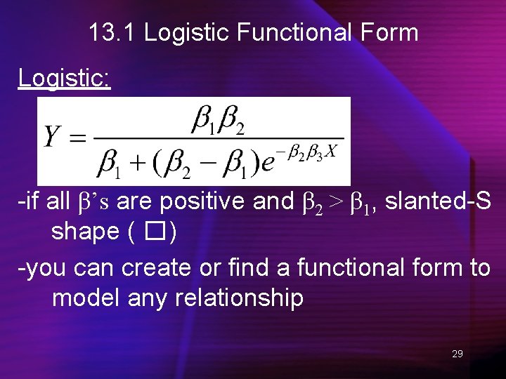
13. 1 Logistic Functional Form Logistic: -if all β’s are positive and β 2 > β 1, slanted-S shape ( �) -you can create or find a functional form to model any relationship 29

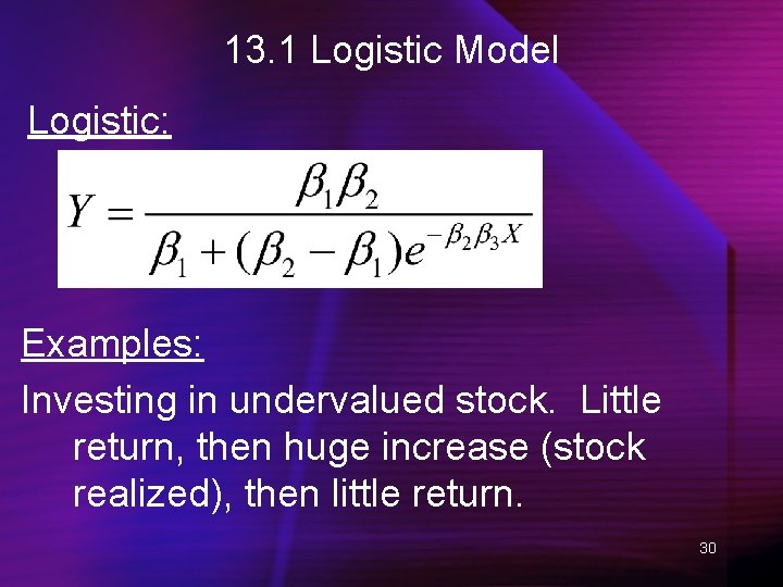
13. 1 Logistic Model Logistic: Examples: Investing in undervalued stock. Little return, then huge increase (stock realized), then little return. 30

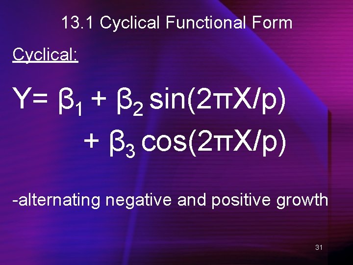
13. 1 Cyclical Functional Form Cyclical: Y= β 1 + β 2 sin(2πX/p) + β 3 cos(2πX/p) -alternating negative and positive growth 31

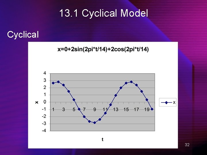
13. 1 Cyclical Model Cyclical 32

13. 1 Cyclical Model Examples: Housing markets Tech markets Oil markets Yearly seasonal markets (fruit, ice cream, etc. ) 33

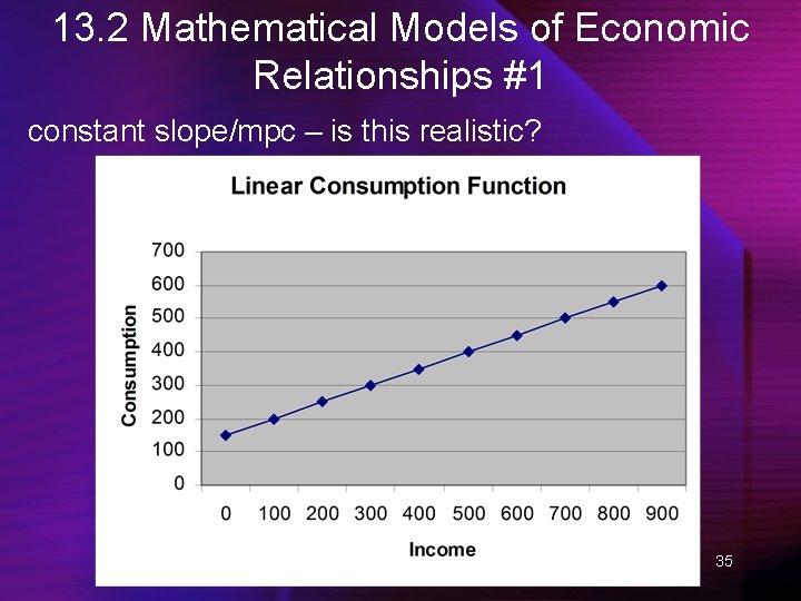
13. 2 Mathematical Models of Economic Relationships #1 Example 1 – Consumption Function -consumption is based on income -even with zero income, some consumption (autonomous consumption) occurs -as income rises, consumption rises -out of every new dollar earned, a fraction, the marginal propensity to consume (mpc) is spent on consumption – remainder is saved -the mpc determines the slope of the graph 34

13. 2 Mathematical Models of Economic Relationships #1 constant slope/mpc – is this realistic? 35

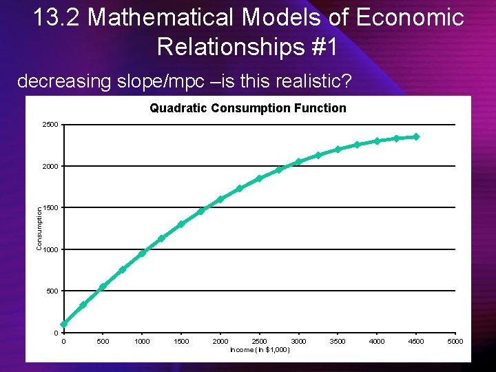
13. 2 Mathematical Models of Economic Relationships #1 decreasing slope/mpc –is this realistic? Quadratic Consumption Function 2500 Consumption 2000 1500 1000 500 0 0 500 1000 1500 2000 2500 3000 Income (In $1, 000) 3500 4000 4500 5000 36

13. 2 Mathematical Models of Economic Relationships #1 Consumption Function – slope = mpc Linear: Consumption = 100+0. 5 income mpc = slope = 0. 5 (constant) Non-Linear Consumption = 100+0. 95 income-0. 001 income 2 mpc = slope = (decreasing) Are any other functional forms viable for consumption? 37

13. 2 Mathematical Models of Economic Relationships #2 Example 2 – Short-run Phillips Curve -if no excess demand in the economy, the economy will be at the natural rate of unemployment -if unemployment falls, wages and prices will tend upwards (hard to find workers) -if unemployment rises, wages and prices will fall (easier to find workers) -these changes are asymmetric (excess labour demand has a bigger effect than excess 38 labour supply)

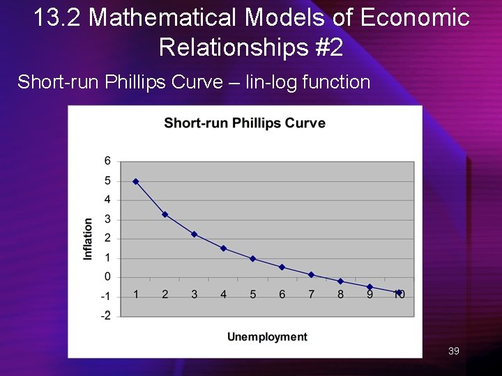
13. 2 Mathematical Models of Economic Relationships #2 Short-run Phillips Curve – lin-log function 39

13. 2 Mathematical Models of Economic Relationships #2 Example 2 – Short-run Phillips Curve Slope = short-run response of inflation to a change in unemployment Inflation = 5 –ln(unemployment) Slope: -as unemployment increases, the slope moves from very negative to slightly negative -there is a greater effect of low unemployment than high unemployment 40

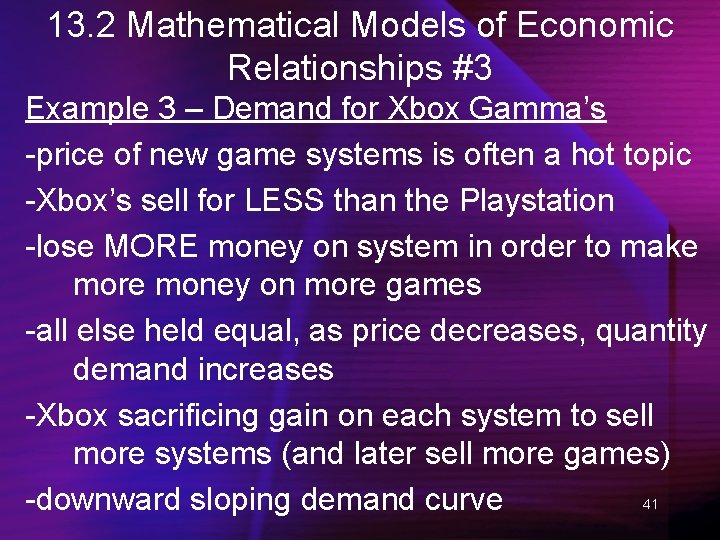
13. 2 Mathematical Models of Economic Relationships #3 Example 3 – Demand for Xbox Gamma’s -price of new game systems is often a hot topic -Xbox’s sell for LESS than the Playstation -lose MORE money on system in order to make more money on more games -all else held equal, as price decreases, quantity demand increases -Xbox sacrificing gain on each system to sell more systems (and later sell more games) 41 -downward sloping demand curve

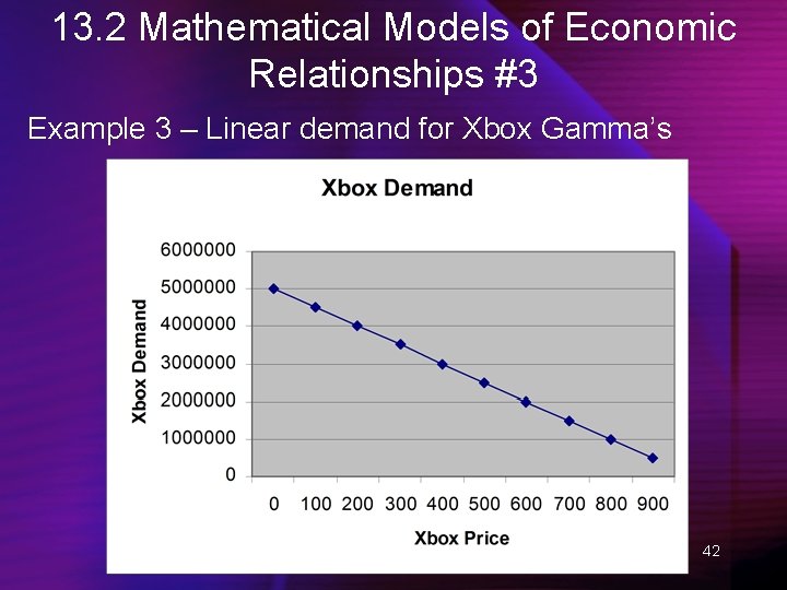
13. 2 Mathematical Models of Economic Relationships #3 Example 3 – Linear demand for Xbox Gamma’s 42

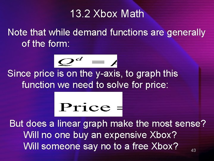
13. 2 Xbox Math Note that while demand functions are generally of the form: Since price is on the y-axis, to graph this function we need to solve for price: But does a linear graph make the most sense? Will no one buy an expensive Xbox? Will someone say no to a free Xbox? 43

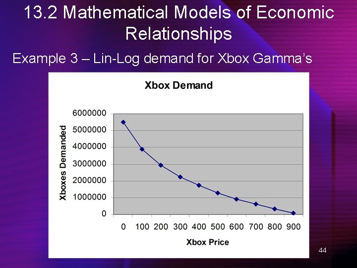
13. 2 Mathematical Models of Economic Relationships Example 3 – Lin-Log demand for Xbox Gamma’s 44

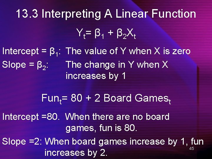
13. 3 Interpreting A Linear Function Y t = β 1 + β 2 X t Intercept = β 1: The value of Y when X is zero Slope = β 2: The change in Y when X increases by 1 Funt= 80 + 2 Board Gamest Intercept =80. When there are no board games, fun is 80. Slope =2: When board games increase by 1, fun 45 increases by 2.

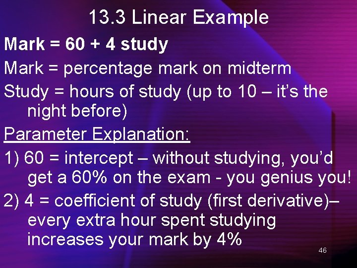
13. 3 Linear Example Mark = 60 + 4 study Mark = percentage mark on midterm Study = hours of study (up to 10 – it’s the night before) Parameter Explanation: 1) 60 = intercept – without studying, you’d get a 60% on the exam - you genius you! 2) 4 = coefficient of study (first derivative)– every extra hour spent studying increases your mark by 4% 46

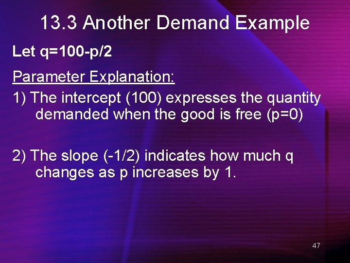
13. 3 Another Demand Example Let q=100 -p/2 Parameter Explanation: 1) The intercept (100) expresses the quantity demanded when the good is free (p=0) 2) The slope (-1/2) indicates how much q changes as p increases by 1. 47

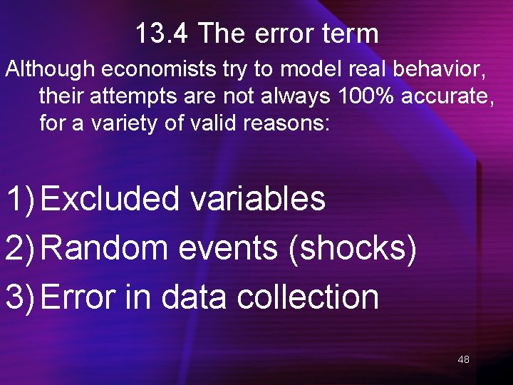
13. 4 The error term Although economists try to model real behavior, their attempts are not always 100% accurate, for a variety of valid reasons: 1) Excluded variables 2) Random events (shocks) 3) Error in data collection 48

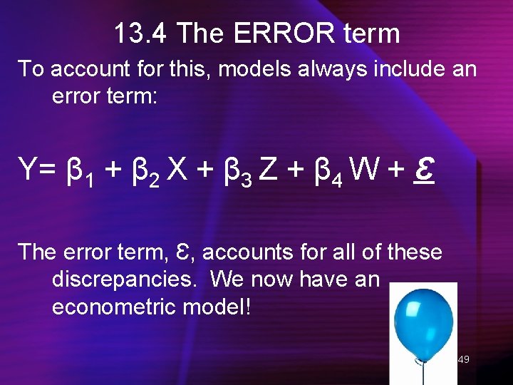
13. 4 The ERROR term To account for this, models always include an error term: Y= β 1 + β 2 X + β 3 Z + β 4 W + Ɛ The error term, Ɛ, accounts for all of these discrepancies. We now have an econometric model! 49

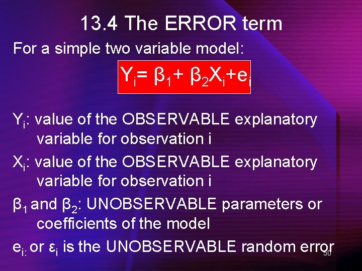
13. 4 The ERROR term For a simple two variable model: Yi= β 1+ β 2 Xi+ei Yi: value of the OBSERVABLE explanatory variable for observation i Xi: value of the OBSERVABLE explanatory variable for observation i β 1 and β 2: UNOBSERVABLE parameters or coefficients of the model ei: or εi is the UNOBSERVABLE random error 50

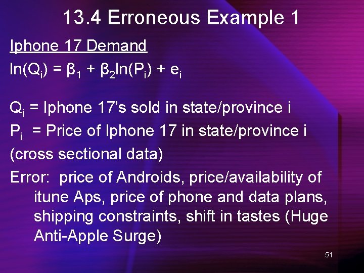
13. 4 Erroneous Example 1 Iphone 17 Demand ln(Qi) = β 1 + β 2 ln(Pi) + ei Qi = Iphone 17’s sold in state/province i Pi = Price of Iphone 17 in state/province i (cross sectional data) Error: price of Androids, price/availability of itune Aps, price of phone and data plans, shipping constraints, shift in tastes (Huge Anti-Apple Surge) 51

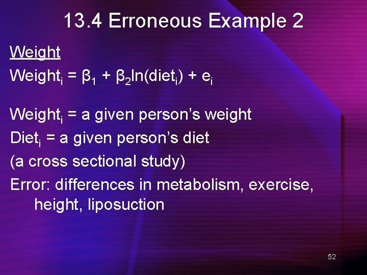
13. 4 Erroneous Example 2 Weighti = β 1 + β 2 ln(dieti) + ei Weighti = a given person’s weight Dieti = a given person’s diet (a cross sectional study) Error: differences in metabolism, exercise, height, liposuction 52

13. 4 Erroneous Example 3 Depressioni = β 1 + β 2 Econmarki + ei Depressioni = level of depression at any point in the course Econmarki = current econ mark (a time series study) Error: quality of last Walking Dead episode, social life, sport team standings, weather, success of Economics pick-up lines 53