13 Determining the Optimal Level of Product Availability
13 Determining the Optimal Level of Product Availability Power. Point presentation to accompany Chopra and Meindl Supply Chain Management, 5 e Copyright © 2013 Pearson Education, Inc. publishing as Prentice Hall. 13 -1 1 -1
Learning Objectives 1. Identify the factors affecting the optimal level of product availability and evaluate the optimal cycle service level 2. Use managerial levers that improve supply chain profitability through optimal service levels 3. Understand conditions under which postponement is valuable in a supply chain 4. Allocate limited supply capacity among multiple products to maximize expected profits Copyright © 2013 Pearson Education, Inc. publishing as Prentice Hall. 13 -2
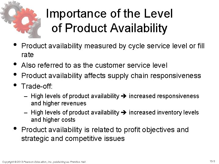
Importance of the Level of Product Availability • • • Product availability measured by cycle service level or fill rate Also referred to as the customer service level Product availability affects supply chain responsiveness Trade-off: – High levels of product availability increased responsiveness and higher revenues – High levels of product availability increased inventory levels and higher costs Product availability is related to profit objectives and strategic and competitive issues Copyright © 2013 Pearson Education, Inc. publishing as Prentice Hall. 13 -3
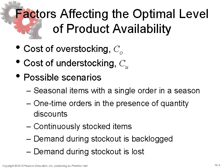
Factors Affecting the Optimal Level of Product Availability • Cost of overstocking, Co • Cost of understocking, Cu • Possible scenarios – Seasonal items with a single order in a season – One-time orders in the presence of quantity discounts – Continuously stocked items – Demand during stockout is backlogged – Demand during stockout is lost Copyright © 2013 Pearson Education, Inc. publishing as Prentice Hall. 13 -4
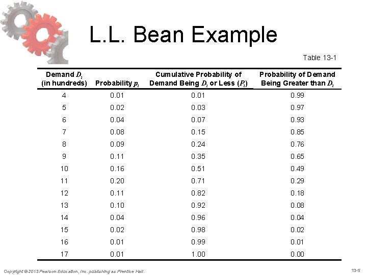
L. L. Bean Example Table 13 -1 Demand Di (in hundreds) Probability pi Cumulative Probability of Demand Being Di or Less (Pi) Probability of Demand Being Greater than Di 4 0. 01 0. 99 5 0. 02 0. 03 0. 97 6 0. 04 0. 07 0. 93 7 0. 08 0. 15 0. 85 8 0. 09 0. 24 0. 76 9 0. 11 0. 35 0. 65 10 0. 16 0. 51 0. 49 11 0. 20 0. 71 0. 29 12 0. 11 0. 82 0. 18 13 0. 10 0. 92 0. 08 14 0. 04 0. 96 0. 04 15 0. 02 0. 98 0. 02 16 0. 01 0. 99 0. 01 17 0. 01 1. 00 0. 00 Copyright © 2013 Pearson Education, Inc. publishing as Prentice Hall. 13 -5
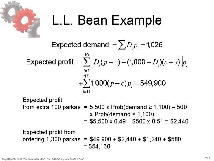
L. L. Bean Example Expected profit from extra 100 parkas = 5, 500 x Prob(demand ≥ 1, 100) – 500 x Prob(demand < 1, 100) = $5, 500 x 0. 49 – $500 x 0. 51 = $2, 440 Expected profit from ordering 1, 300 parkas = $49, 900 + $2, 440 + $1, 240 + $580 = $54, 160 Copyright © 2013 Pearson Education, Inc. publishing as Prentice Hall. 13 -6
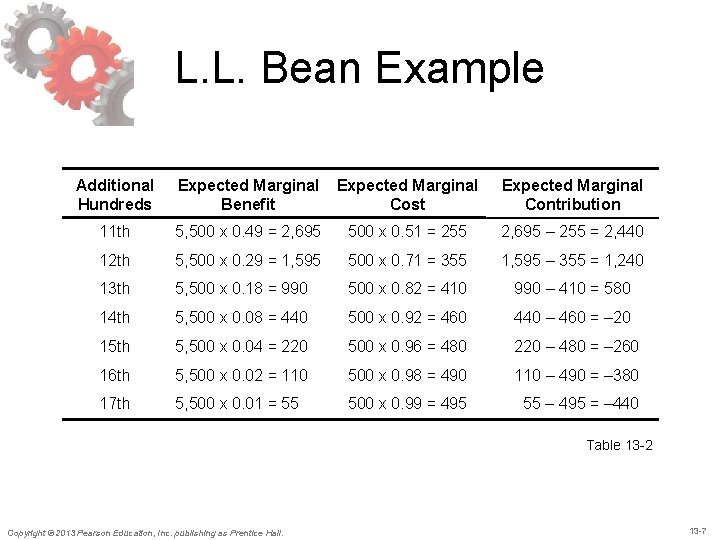
L. L. Bean Example Additional Hundreds Expected Marginal Benefit Expected Marginal Cost Expected Marginal Contribution 11 th 5, 500 x 0. 49 = 2, 695 500 x 0. 51 = 255 2, 695 – 255 = 2, 440 12 th 5, 500 x 0. 29 = 1, 595 500 x 0. 71 = 355 1, 595 – 355 = 1, 240 13 th 5, 500 x 0. 18 = 990 500 x 0. 82 = 410 990 – 410 = 580 14 th 5, 500 x 0. 08 = 440 500 x 0. 92 = 460 440 – 460 = – 20 15 th 5, 500 x 0. 04 = 220 500 x 0. 96 = 480 220 – 480 = – 260 16 th 5, 500 x 0. 02 = 110 500 x 0. 98 = 490 110 – 490 = – 380 17 th 5, 500 x 0. 01 = 55 500 x 0. 99 = 495 55 – 495 = – 440 Table 13 -2 Copyright © 2013 Pearson Education, Inc. publishing as Prentice Hall. 13 -7
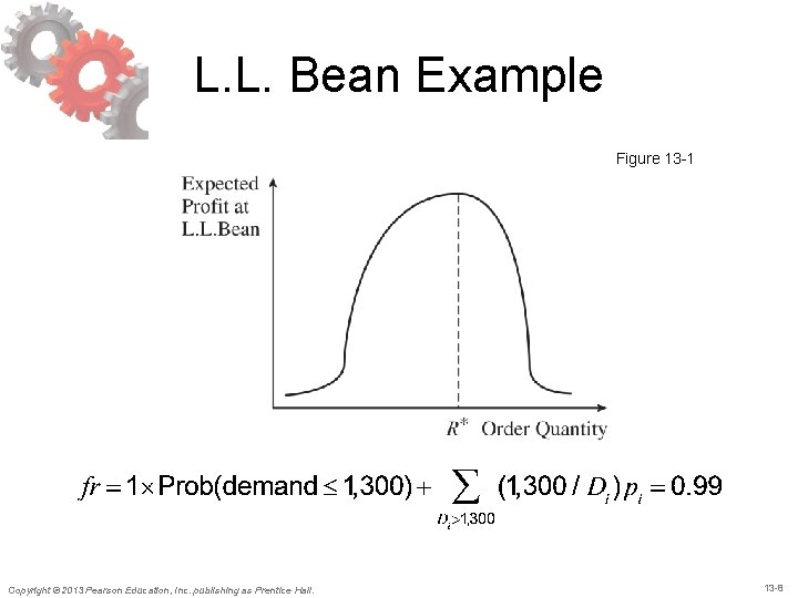
L. L. Bean Example Figure 13 -1 Copyright © 2013 Pearson Education, Inc. publishing as Prentice Hall. 13 -8
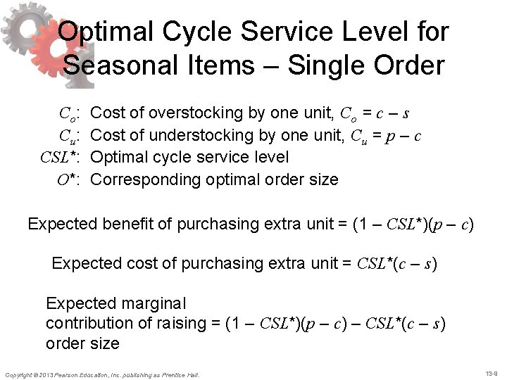
Optimal Cycle Service Level for Seasonal Items – Single Order Co: Cu: CSL*: O*: Cost of overstocking by one unit, Co = c – s Cost of understocking by one unit, Cu = p – c Optimal cycle service level Corresponding optimal order size Expected benefit of purchasing extra unit = (1 – CSL*)(p – c) Expected cost of purchasing extra unit = CSL*(c – s) Expected marginal contribution of raising = (1 – CSL*)(p – c) – CSL*(c – s) order size Copyright © 2013 Pearson Education, Inc. publishing as Prentice Hall. 13 -9
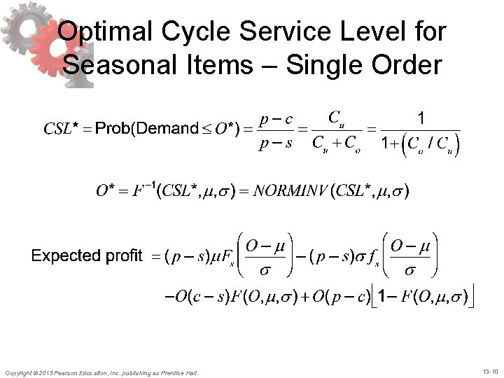
Optimal Cycle Service Level for Seasonal Items – Single Order Copyright © 2013 Pearson Education, Inc. publishing as Prentice Hall. 13 -10
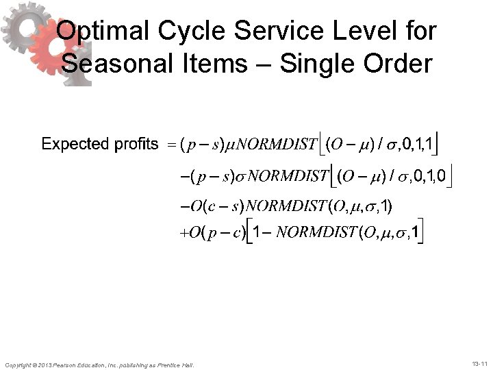
Optimal Cycle Service Level for Seasonal Items – Single Order Copyright © 2013 Pearson Education, Inc. publishing as Prentice Hall. 13 -11
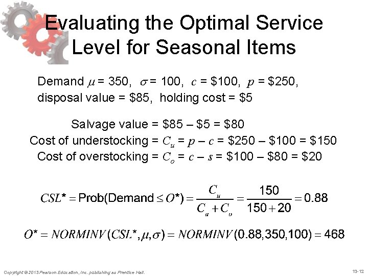
Evaluating the Optimal Service Level for Seasonal Items Demand m = 350, = 100, c = $100, p = $250, disposal value = $85, holding cost = $5 Salvage value = $85 – $5 = $80 Cost of understocking = Cu = p – c = $250 – $100 = $150 Cost of overstocking = Co = c – s = $100 – $80 = $20 Copyright © 2013 Pearson Education, Inc. publishing as Prentice Hall. 13 -12
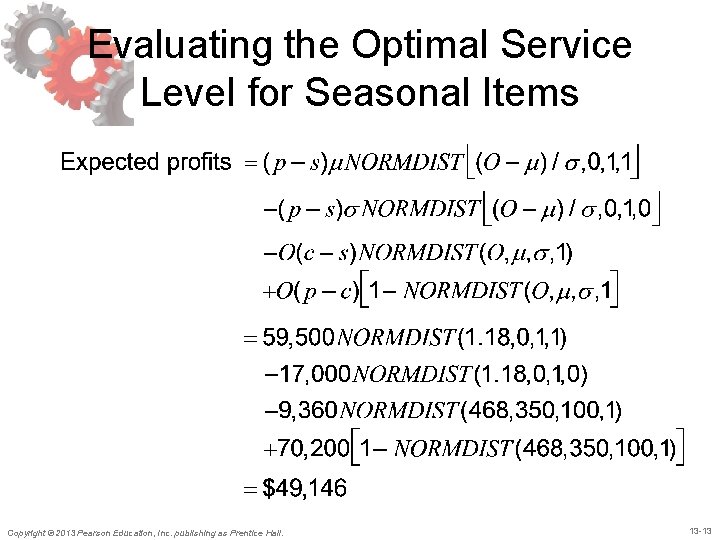
Evaluating the Optimal Service Level for Seasonal Items Copyright © 2013 Pearson Education, Inc. publishing as Prentice Hall. 13 -13
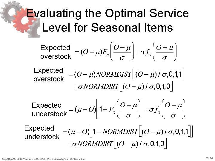
Evaluating the Optimal Service Level for Seasonal Items Expected overstock Expected understock Copyright © 2013 Pearson Education, Inc. publishing as Prentice Hall. 13 -14
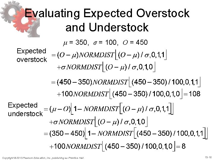
Evaluating Expected Overstock and Understock μ = 350, σ = 100, O = 450 Expected overstock Expected understock Copyright © 2013 Pearson Education, Inc. publishing as Prentice Hall. 13 -15
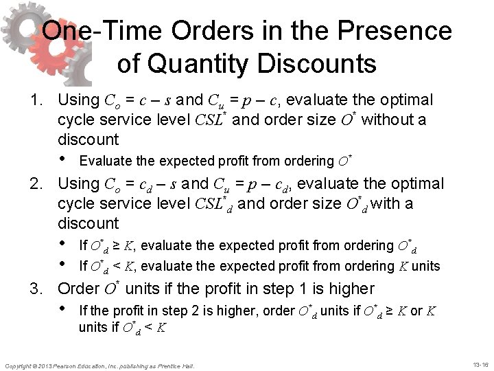
One-Time Orders in the Presence of Quantity Discounts 1. Using Co = c – s and Cu = p – c, evaluate the optimal cycle service level CSL* and order size O* without a discount • Evaluate the expected profit from ordering O* 2. Using Co = cd – s and Cu = p – cd, evaluate the optimal cycle service level CSL*d and order size O*d with a discount • • If O*d ≥ K, evaluate the expected profit from ordering O*d If O*d < K, evaluate the expected profit from ordering K units 3. Order O* units if the profit in step 1 is higher • If the profit in step 2 is higher, order O*d units if O*d ≥ K or K units if O*d < K Copyright © 2013 Pearson Education, Inc. publishing as Prentice Hall. 13 -16
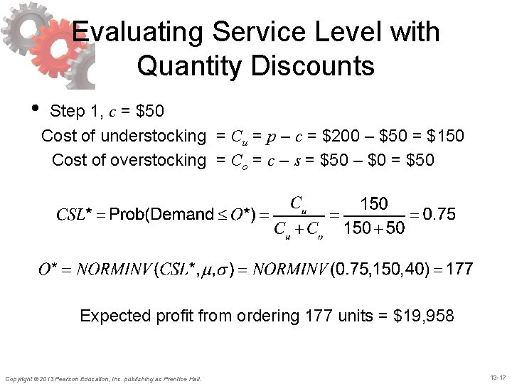
Evaluating Service Level with Quantity Discounts • Step 1, c = $50 Cost of understocking = Cu = p – c = $200 – $50 = $150 Cost of overstocking = Co = c – s = $50 – $0 = $50 Expected profit from ordering 177 units = $19, 958 Copyright © 2013 Pearson Education, Inc. publishing as Prentice Hall. 13 -17
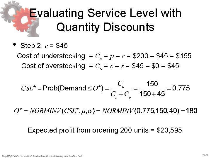
Evaluating Service Level with Quantity Discounts • Step 2, c = $45 Cost of understocking = Cu = p – c = $200 – $45 = $155 Cost of overstocking = Co = c – s = $45 – $0 = $45 Expected profit from ordering 200 units = $20, 595 Copyright © 2013 Pearson Education, Inc. publishing as Prentice Hall. 13 -18
Desired Cycle Service Level for Continuously Stocked Items • Two extreme scenarios 1. All demand that arises when the product is out of stock is backlogged and filled later, when inventories are replenished 2. All demand arising when the product is out of stock is lost Copyright © 2013 Pearson Education, Inc. publishing as Prentice Hall. 13 -19
Desired Cycle Service Level for Continuously Stocked Items Q: Replenishment lot size S: Fixed cost associated with each order ROP: Reorder point D: Average demand per unit time σ : Standard deviation of demand per unit time ss: Safety inventory (ss = ROP – DL) CSL: Cycle service level C: Unit cost h: Holding cost as a fraction of product cost per unit time H: Cost of holding one unit for one unit of time. H = h. C Copyright © 2013 Pearson Education, Inc. publishing as Prentice Hall. 13 -20
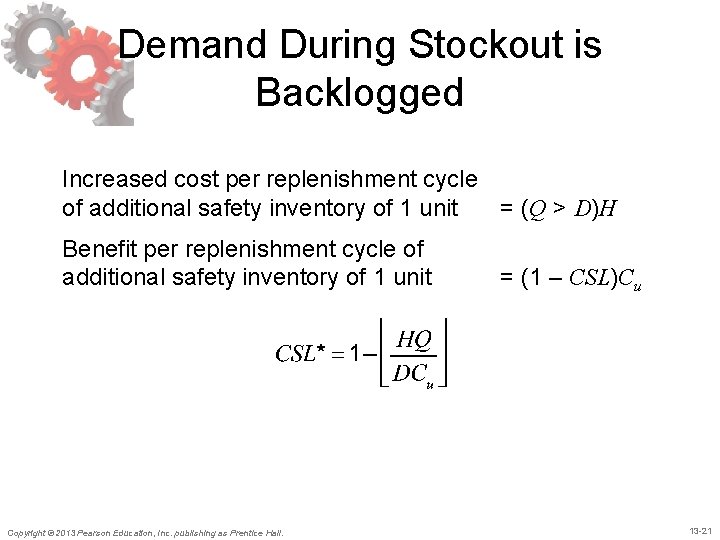
Demand During Stockout is Backlogged Increased cost per replenishment cycle of additional safety inventory of 1 unit = (Q > D)H Benefit per replenishment cycle of additional safety inventory of 1 unit Copyright © 2013 Pearson Education, Inc. publishing as Prentice Hall. = (1 – CSL)Cu 13 -21
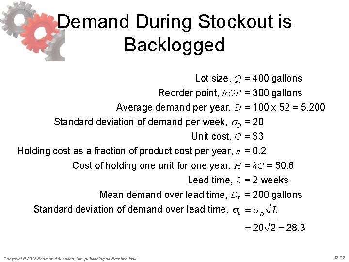
Demand During Stockout is Backlogged Lot size, Q = 400 gallons Reorder point, ROP = 300 gallons Average demand per year, D = 100 x 52 = 5, 200 Standard deviation of demand per week, D Unit cost, C Holding cost as a fraction of product cost per year, h Cost of holding one unit for one year, H Lead time, L Mean demand over lead time, DL = 20 = $3 = 0. 2 = h. C = $0. 6 = 2 weeks = 200 gallons Standard deviation of demand over lead time, L Copyright © 2013 Pearson Education, Inc. publishing as Prentice Hall. 13 -22
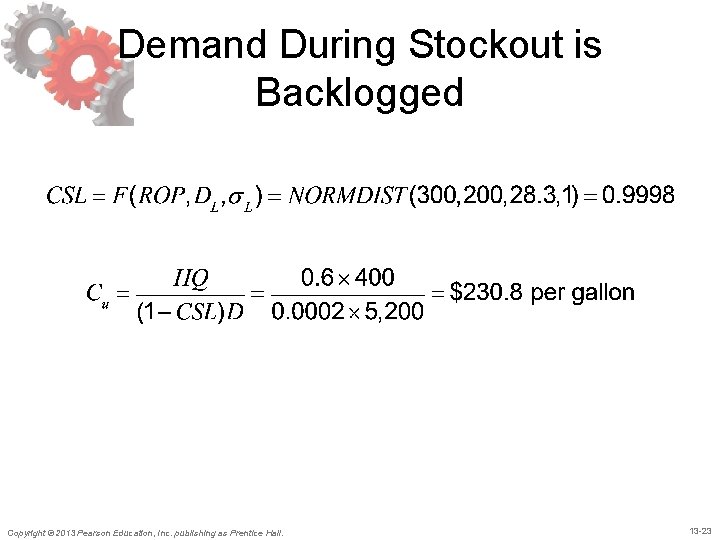
Demand During Stockout is Backlogged Copyright © 2013 Pearson Education, Inc. publishing as Prentice Hall. 13 -23
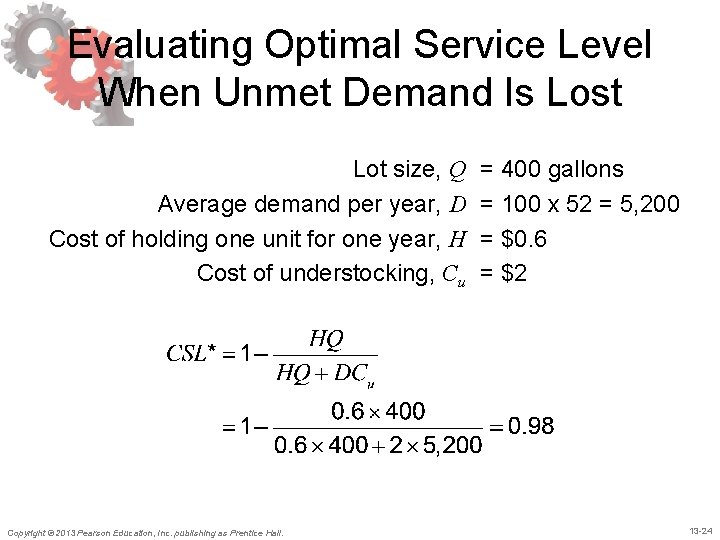
Evaluating Optimal Service Level When Unmet Demand Is Lost Lot size, Q Average demand per year, D Cost of holding one unit for one year, H Cost of understocking, Cu Copyright © 2013 Pearson Education, Inc. publishing as Prentice Hall. = 400 gallons = 100 x 52 = 5, 200 = $0. 6 = $2 13 -24
Managerial Levers to Improve Supply Chain Profitability • “Obvious” actions 1. Increase salvage value of each unit 2. Decrease the margin lost from a stockout • Improved forecasting • Quick response • Postponement • Tailored sourcing Copyright © 2013 Pearson Education, Inc. publishing as Prentice Hall. 13 -25
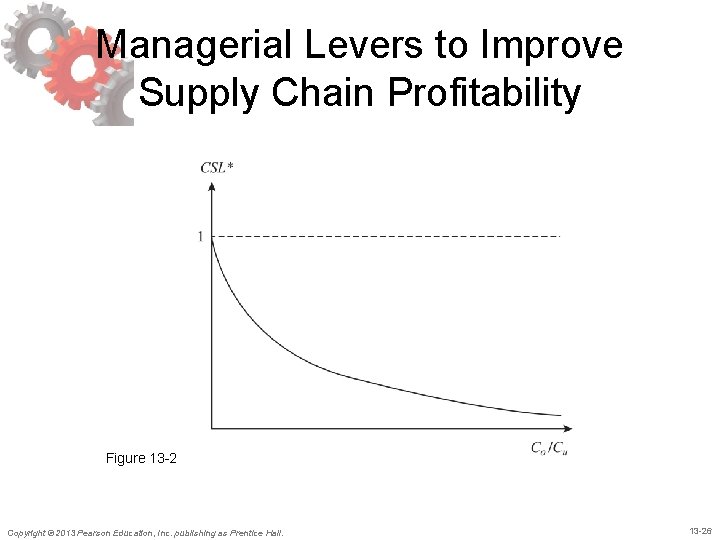
Managerial Levers to Improve Supply Chain Profitability Figure 13 -2 Copyright © 2013 Pearson Education, Inc. publishing as Prentice Hall. 13 -26
Improved Forecasts • Improved forecasts result in reduced • uncertainty Less uncertainty results in – Lower levels of safety inventory (and costs) for the same level of product availability, or – Higher product availability for the same level of safety inventory, or – Both Copyright © 2013 Pearson Education, Inc. publishing as Prentice Hall. 13 -27
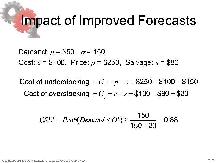
Impact of Improved Forecasts Demand: m = 350, = 150 Cost: c = $100, Price: p = $250, Salvage: s = $80 Copyright © 2013 Pearson Education, Inc. publishing as Prentice Hall. 13 -28
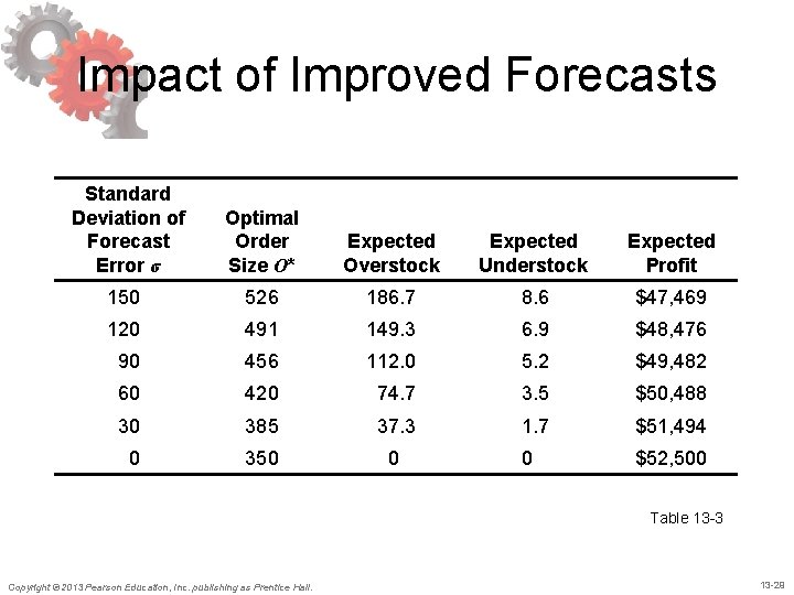
Impact of Improved Forecasts Standard Deviation of Forecast Error σ Optimal Order Size O* Expected Overstock Expected Understock Expected Profit 150 526 186. 7 8. 6 $47, 469 120 491 149. 3 6. 9 $48, 476 90 456 112. 0 5. 2 $49, 482 60 420 74. 7 3. 5 $50, 488 30 385 37. 3 1. 7 $51, 494 0 350 0 0 $52, 500 Table 13 -3 Copyright © 2013 Pearson Education, Inc. publishing as Prentice Hall. 13 -29
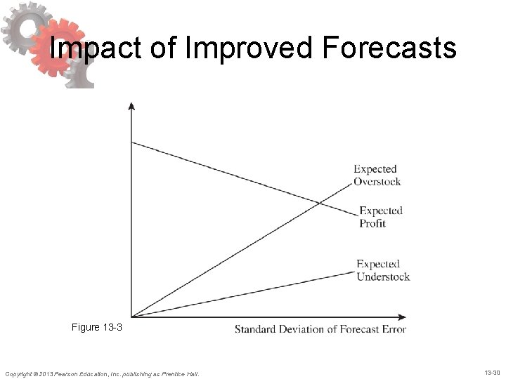
Impact of Improved Forecasts Figure 13 -3 Copyright © 2013 Pearson Education, Inc. publishing as Prentice Hall. 13 -30
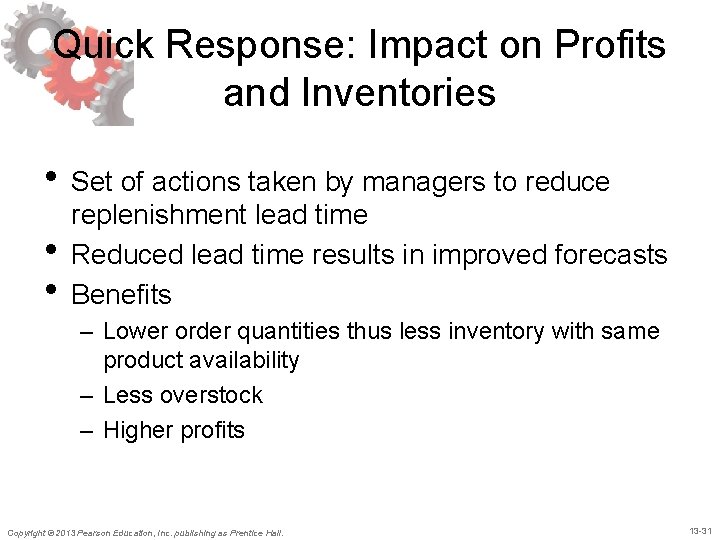
Quick Response: Impact on Profits and Inventories • Set of actions taken by managers to reduce • • replenishment lead time Reduced lead time results in improved forecasts Benefits – Lower order quantities thus less inventory with same product availability – Less overstock – Higher profits Copyright © 2013 Pearson Education, Inc. publishing as Prentice Hall. 13 -31
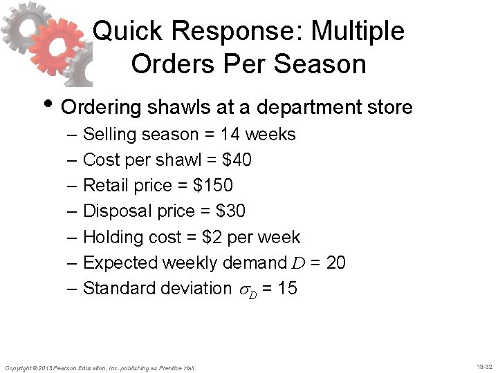
Quick Response: Multiple Orders Per Season • Ordering shawls at a department store – Selling season = 14 weeks – Cost per shawl = $40 – Retail price = $150 – Disposal price = $30 – Holding cost = $2 per week – Expected weekly demand D = 20 – Standard deviation D = 15 Copyright © 2013 Pearson Education, Inc. publishing as Prentice Hall. 13 -32
Quick Response: Multiple Orders Per Season • Two ordering policies 1. Supply lead time is more than 15 weeks • Single order placed at the beginning of the season • Supply lead time is reduced to six weeks 2. Two orders are placed for the season • One for delivery at the beginning of the season • One at the end of week 1 for delivery in week 8 Copyright © 2013 Pearson Education, Inc. publishing as Prentice Hall. 13 -33
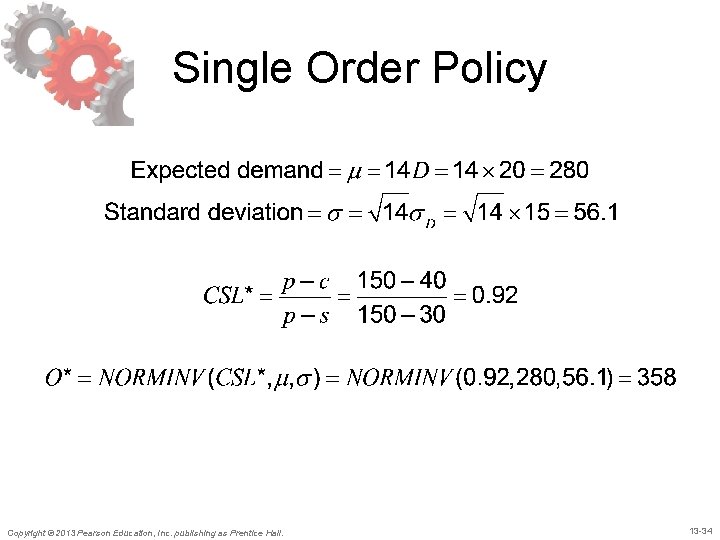
Single Order Policy Copyright © 2013 Pearson Education, Inc. publishing as Prentice Hall. 13 -34
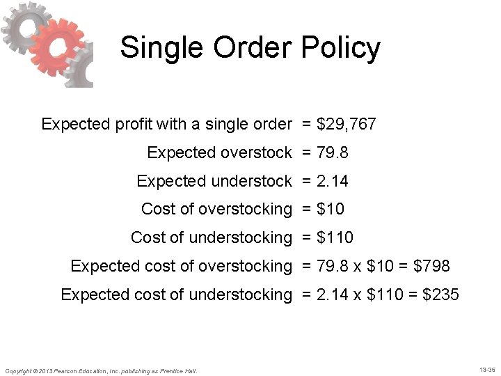
Single Order Policy Expected profit with a single order = $29, 767 Expected overstock = 79. 8 Expected understock = 2. 14 Cost of overstocking = $10 Cost of understocking = $110 Expected cost of overstocking = 79. 8 x $10 = $798 Expected cost of understocking = 2. 14 x $110 = $235 Copyright © 2013 Pearson Education, Inc. publishing as Prentice Hall. 13 -35
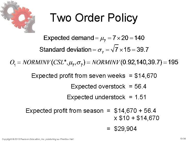
Two Order Policy Expected profit from seven weeks = $14, 670 Expected overstock = 56. 4 Expected understock = 1. 51 Expected profit from season = $14, 670 + 56. 4 x $10 + $14, 670 = $29, 904 Copyright © 2013 Pearson Education, Inc. publishing as Prentice Hall. 13 -36
Quick Response: Multiple Orders Per Season • Three important consequences 1. The expected total quantity ordered during the season with two orders is less than that with a single order for the same cycle service level 2. The average overstock to be disposed of at the end of the sales season is less if a follow-up order is allowed after observing some sales 3. The profits are higher when a follow-up order is allowed during the sales season Copyright © 2013 Pearson Education, Inc. publishing as Prentice Hall. 13 -37
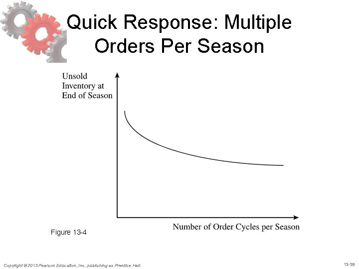
Quick Response: Multiple Orders Per Season Figure 13 -4 Copyright © 2013 Pearson Education, Inc. publishing as Prentice Hall. 13 -38
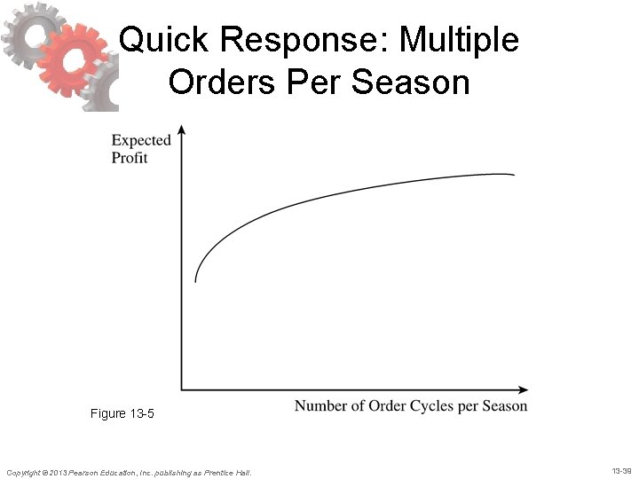
Quick Response: Multiple Orders Per Season Figure 13 -5 Copyright © 2013 Pearson Education, Inc. publishing as Prentice Hall. 13 -39
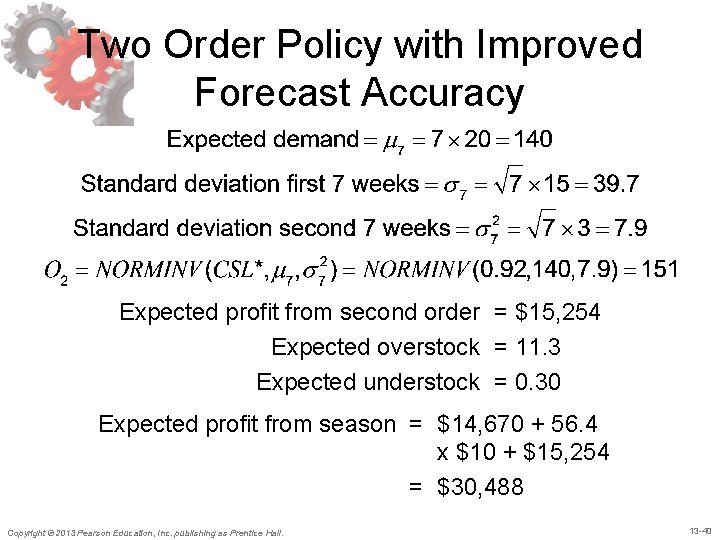
Two Order Policy with Improved Forecast Accuracy Expected profit from second order = $15, 254 Expected overstock = 11. 3 Expected understock = 0. 30 Expected profit from season = $14, 670 + 56. 4 x $10 + $15, 254 = $30, 488 Copyright © 2013 Pearson Education, Inc. publishing as Prentice Hall. 13 -40
Postponement: Impact on Profits and Inventories • Delay of product differentiation until closer to • • • the sale of the product Activities prior to product differentiation require aggregate forecasts more accurate than individual product forecasts Individual product forecasts are needed close to the time of sale Results in a better match of supply and demand Valuable in online sales Higher profits through better matching of supply and demand Copyright © 2013 Pearson Education, Inc. publishing as Prentice Hall. 13 -41
Value of Postponement: Benetton For each of four colors Demand m = 1, 000, = 50, Sale price p = $50, Salvage value s = $10 Production cost Option 1 (no postponement) = $20 Production cost Option 2 (postponement) = $22 Copyright © 2013 Pearson Education, Inc. publishing as Prentice Hall. 13 -42
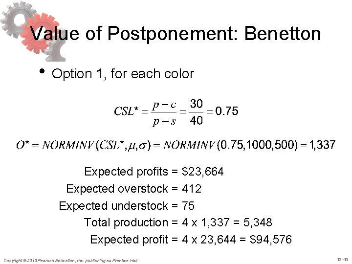
Value of Postponement: Benetton • Option 1, for each color Expected profits = $23, 664 Expected overstock = 412 Expected understock = 75 Total production = 4 x 1, 337 = 5, 348 Expected profit = 4 x 23, 644 = $94, 576 Copyright © 2013 Pearson Education, Inc. publishing as Prentice Hall. 13 -43
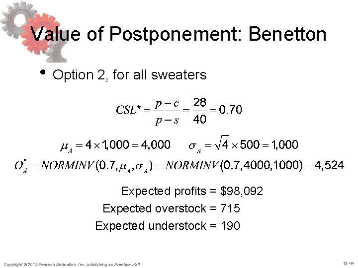
Value of Postponement: Benetton • Option 2, for all sweaters Expected profits = $98, 092 Expected overstock = 715 Expected understock = 190 Copyright © 2013 Pearson Education, Inc. publishing as Prentice Hall. 13 -44
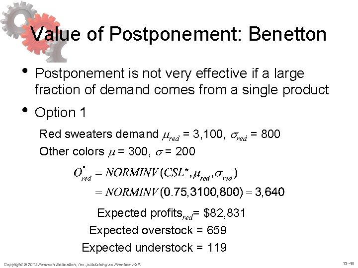
Value of Postponement: Benetton • Postponement is not very effective if a large fraction of demand comes from a single product • Option 1 Red sweaters demand mred = 3, 100, red = 800 Other colors m = 300, = 200 Expected profitsred= $82, 831 Expected overstock = 659 Expected understock = 119 Copyright © 2013 Pearson Education, Inc. publishing as Prentice Hall. 13 -45
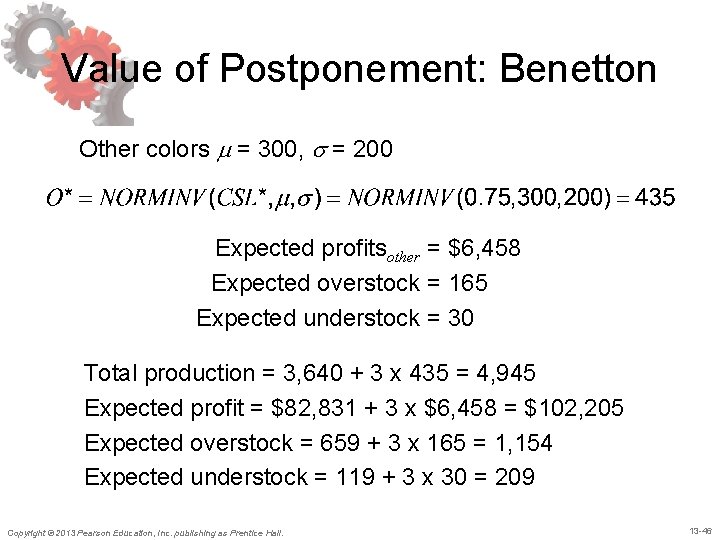
Value of Postponement: Benetton Other colors m = 300, = 200 Expected profitsother = $6, 458 Expected overstock = 165 Expected understock = 30 Total production = 3, 640 + 3 x 435 = 4, 945 Expected profit = $82, 831 + 3 x $6, 458 = $102, 205 Expected overstock = 659 + 3 x 165 = 1, 154 Expected understock = 119 + 3 x 30 = 209 Copyright © 2013 Pearson Education, Inc. publishing as Prentice Hall. 13 -46
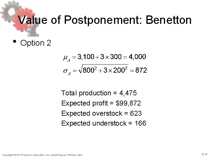
Value of Postponement: Benetton • Option 2 Total production = 4, 475 Expected profit = $99, 872 Expected overstock = 623 Expected understock = 166 Copyright © 2013 Pearson Education, Inc. publishing as Prentice Hall. 13 -47
Tailored Postponement: Benetton • Use production with postponement to satisfy • a part of demand, the rest without postponement Produce red sweaters without postponement, postpone all others Profit = $103, 213 • Tailored postponement allows a firm to increase profits by postponing differentiation only for products with uncertain demand Copyright © 2013 Pearson Education, Inc. publishing as Prentice Hall. 13 -48
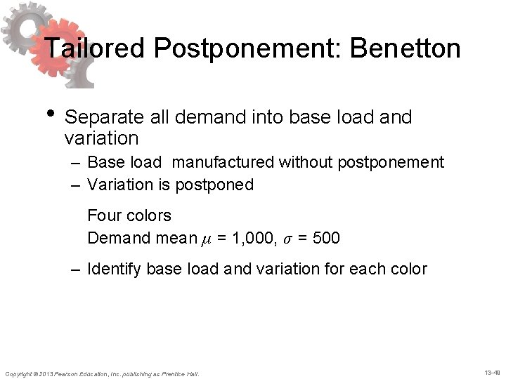
Tailored Postponement: Benetton • Separate all demand into base load and variation – Base load manufactured without postponement – Variation is postponed Four colors Demand mean μ = 1, 000, σ = 500 – Identify base load and variation for each color Copyright © 2013 Pearson Education, Inc. publishing as Prentice Hall. 13 -49
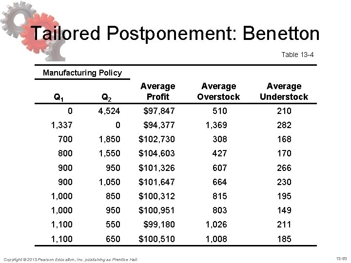
Tailored Postponement: Benetton Table 13 -4 Manufacturing Policy Q 1 Q 2 Average Profit Average Overstock Average Understock 0 4, 524 $97, 847 510 210 1, 337 0 $94, 377 1, 369 282 700 1, 850 $102, 730 308 168 800 1, 550 $104, 603 427 170 900 950 $101, 326 607 266 900 1, 050 $101, 647 664 230 1, 000 850 $100, 312 815 195 1, 000 950 $100, 951 803 149 1, 100 550 $99, 180 1, 026 211 1, 100 650 $100, 510 1, 008 185 Copyright © 2013 Pearson Education, Inc. publishing as Prentice Hall. 13 -50
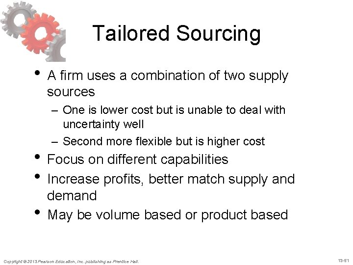
Tailored Sourcing • A firm uses a combination of two supply sources – One is lower cost but is unable to deal with uncertainty well – Second more flexible but is higher cost • Focus on different capabilities • Increase profits, better match supply and • demand May be volume based or product based Copyright © 2013 Pearson Education, Inc. publishing as Prentice Hall. 13 -51
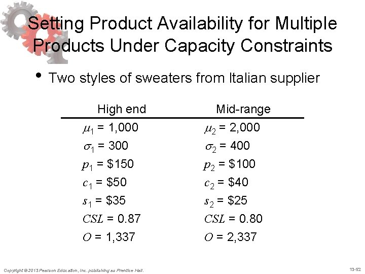
Setting Product Availability for Multiple Products Under Capacity Constraints • Two styles of sweaters from Italian supplier High end m 1 = 1, 000 1 = 300 p 1 = $150 Mid-range m 2 = 2, 000 2 = 400 p 2 = $100 c 1 = $50 s 1 = $35 CSL = 0. 87 O = 1, 337 c 2 = $40 s 2 = $25 CSL = 0. 80 O = 2, 337 Copyright © 2013 Pearson Education, Inc. publishing as Prentice Hall. 13 -52
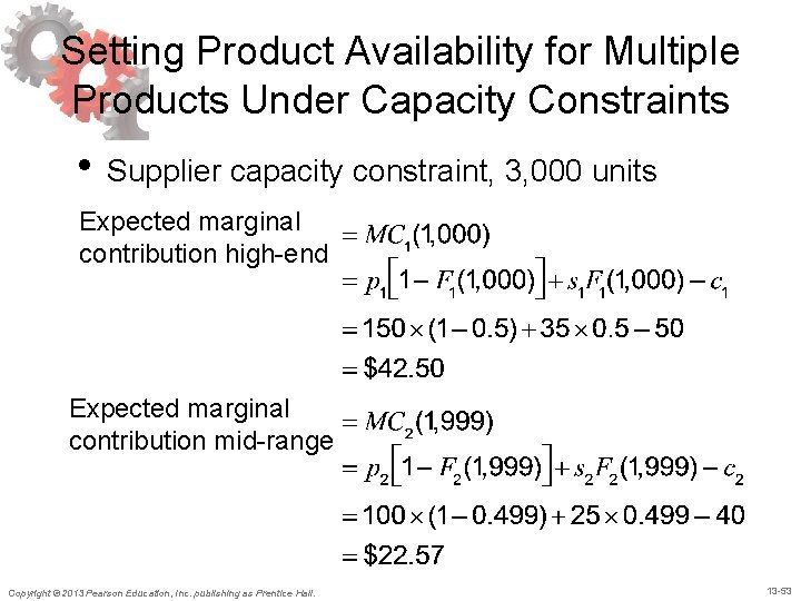
Setting Product Availability for Multiple Products Under Capacity Constraints • Supplier capacity constraint, 3, 000 units Expected marginal contribution high-end Expected marginal contribution mid-range Copyright © 2013 Pearson Education, Inc. publishing as Prentice Hall. 13 -53
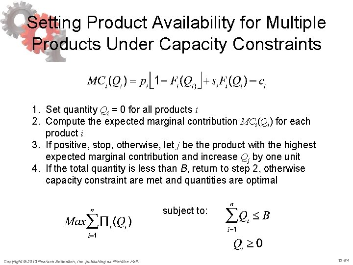
Setting Product Availability for Multiple Products Under Capacity Constraints 1. Set quantity Qi = 0 for all products i 2. Compute the expected marginal contribution MCi(Qi) for each product i 3. If positive, stop, otherwise, let j be the product with the highest expected marginal contribution and increase Qj by one unit 4. If the total quantity is less than B, return to step 2, otherwise capacity constraint are met and quantities are optimal subject to: Copyright © 2013 Pearson Education, Inc. publishing as Prentice Hall. 13 -54
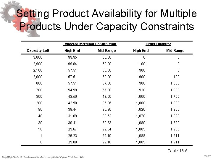
Setting Product Availability for Multiple Products Under Capacity Constraints Expected Marginal Contribution Order Quantity Capacity Left High End Mid Range 3, 000 99. 95 60. 00 0 0 2, 900 99. 84 60. 00 100 0 2, 100 57. 51 60. 00 900 0 2, 000 57. 51 60. 00 900 100 800 57. 51 57. 00 900 1, 300 780 54. 59 57. 00 920 1, 300 42. 50 43. 00 1, 000 1, 700 200 42. 50 36. 86 1, 000 1, 800 180 39. 44 36. 86 1, 020 1, 800 40 31. 89 30. 63 1, 070 1, 890 30 30. 41 30. 63 1, 080 1, 890 10 29. 67 29. 54 1, 085 1, 905 1 29. 23 29. 10 1, 088 1, 911 0 29. 09 29. 10 1, 089 1, 911 Table 13 -5 Copyright © 2013 Pearson Education, Inc. publishing as Prentice Hall. 13 -55
Setting Optimal Levels of Product Availability in Practice 1. Beware of preset levels of availability 2. Use approximate costs because profitmaximizing solutions are quite robust 3. Estimate a range for the cost of stocking out 4. Tailor your response to uncertainty Copyright © 2013 Pearson Education, Inc. publishing as Prentice Hall. 13 -56
Summary of Learning Objectives 1. Identify the factors affecting the optimal level of product availability and evaluate the optimal cycle service level 2. Use managerial levers that improve supply chain profitability through optimal service levels 3. Understand conditions under which postponement is valuable in a supply chain 4. Allocate limited supply capacity among multiple products to maximize expected profits Copyright © 2013 Pearson Education, Inc. publishing as Prentice Hall. 13 -57

All rights reserved. No part of this publication may be reproduced, stored in a retrieval system, or transmitted, in any form or by any means, electronic, mechanical, photocopying, recording, or otherwise, without the prior written permission of the publisher. Printed in the United States of America. Copyright © 2013 Pearson Education, Inc. publishing as Prentice Hall. 13 -58
- Slides: 58