12 Inventory Management 2011 Pearson Education Inc publishing
12 Inventory Management © 2011 Pearson Education, Inc. publishing as Prentice Hall 12 - 1
Outline u The Importance of Inventory u Functions of Inventory u Types of Inventory u Independent vs. Dependent Demand u Managing Inventory u ABC Analysis u Record Accuracy u Cycle Counting u Control of Service Inventories © 2011 Pearson Education, Inc. publishing as Prentice Hall 12 - 2
Outline – Continued u Inventory Models for Independent Demand u. The Basic Economic Order Quantity (EOQ) Model u. Production Order Quantity (POQ) Model u. Quantity Discount Models © 2011 Pearson Education, Inc. publishing as Prentice Hall 12 - 3

Amazon. com u Amazon. com started as a “virtual” retailer – no inventory, no warehouses, no overhead; just computers taking orders to be filled by others u Growth has forced Amazon. com to become a world leader in warehousing and inventory management © 2011 Pearson Education, Inc. publishing as Prentice Hall 12 - 4
Inventory Management The objective of inventory management is to strike a balance between inventory investment and customer service © 2011 Pearson Education, Inc. publishing as Prentice Hall 12 - 5

Inventory Classifications Inventory Proces s stage Raw Material WIP Finished Goods Number & Value A Items B Items C Items Deman d Type Independen t Dependent Other Maintenanc e Repair Operating 12 - 6
Independent Versus Dependent Demand u Independent demand - the demand for the item is independent of the demand for any other item in inventory u Dependent demand - the demand for the item is dependent upon the demand for some other item in the inventory © 2011 Pearson Education, Inc. publishing as Prentice Hall 12 - 7
Examples for Independent Versus Dependent Demand u Independent demand – finished goods, items that are ready to be sold u E. g. computers, cars, u Dependent demand – components of finished products u E. g. parts such as chip, and engine that make up these finished goods 8 12 - 8
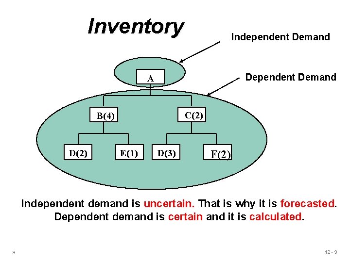
Inventory Independent Demand Dependent Demand A C(2) B(4) D(2) E(1) D(3) F(2) Independent demand is uncertain. That is why it is forecasted. Dependent demand is certain and it is calculated. 9 12 - 9
Functions of Inventory 1. To decouple or separate various parts of the production process 2. To protect the company against fluctuations in demand provide a stock of goods that will provide a selection for customers 3. To take advantage of quantity discounts 4. To hedge against inflation © 2011 Pearson Education, Inc. publishing as Prentice Hall 12 - 10
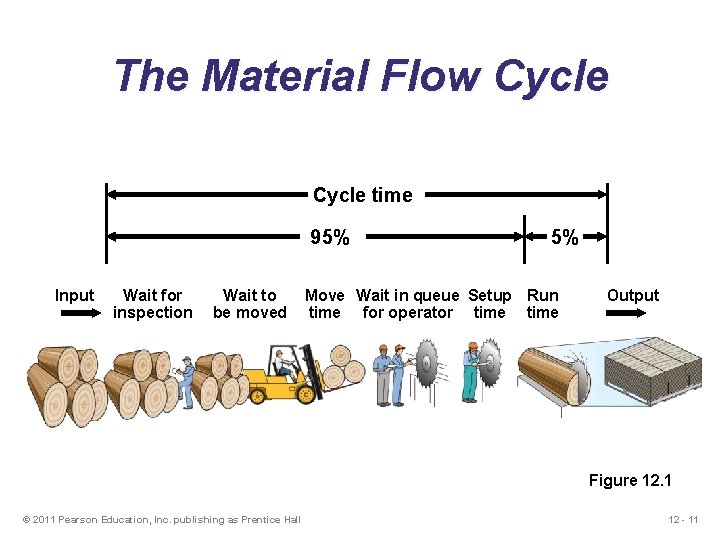
The Material Flow Cycle time 95% Input Wait for inspection Wait to be moved 5% Move Wait in queue Setup Run time for operator time Output Figure 12. 1 © 2011 Pearson Education, Inc. publishing as Prentice Hall 12 - 11
Importance of Inventory u One of the most expensive assets of many companies representing as much as 50% of total invested capital u Operations managers must balance inventory investment and customer service © 2011 Pearson Education, Inc. publishing as Prentice Hall 12 - 12
Important Issues in Inventory Management 1. Classifying inventory items 2. Keeping accurate inventory records © 2011 Pearson Education, Inc. publishing as Prentice Hall 12 - 13
Multiproduct Systems: A-B-C Analysis (It is based on the principles of ‘vital few and trivial many’) u Vilfredo Pareto studied the distribution of wealth in 19 th century and noted that large portion of the wealth is owned by small segment of the population. u Typically the top 20% of the items account for the 80% of the annual dollar value of sales, the next 30 percent for the next 15. © 2011 Pearson Education, Inc. publishing as Prentice Hall 12 - 14
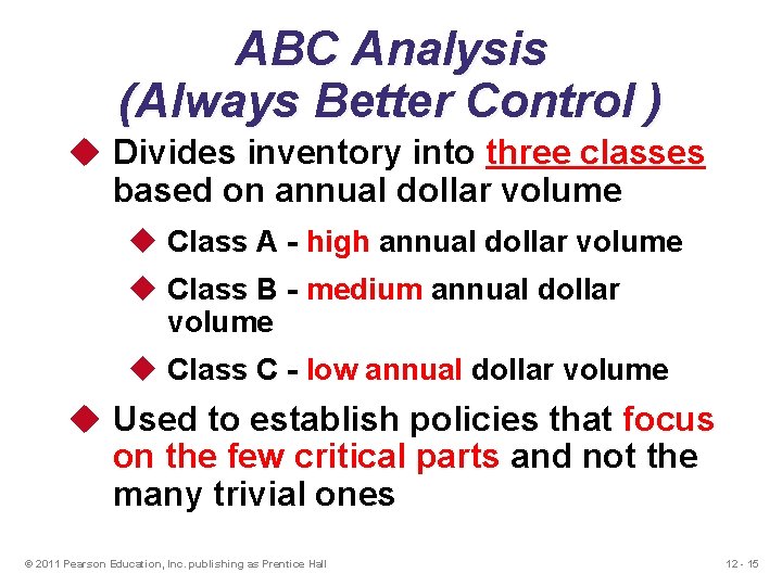
ABC Analysis (Always Better Control ) u Divides inventory into three classes based on annual dollar volume u Class A - high annual dollar volume u Class B - medium annual dollar volume u Class C - low annual dollar volume u Used to establish policies that focus on the few critical parts and not the many trivial ones © 2011 Pearson Education, Inc. publishing as Prentice Hall 12 - 15
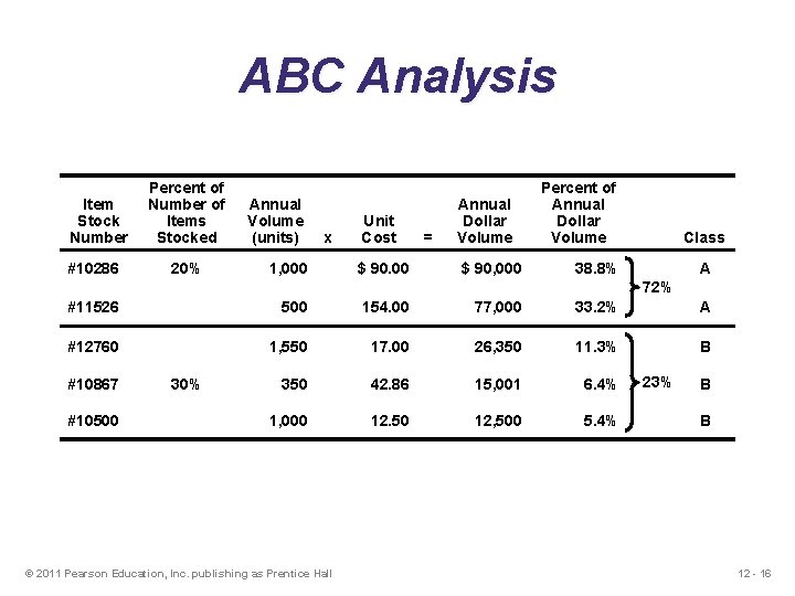
ABC Analysis Item Stock Number #10286 Percent of Number of Items Stocked 20% Annual Volume (units) x 1, 000 Unit Cost $ 90. 00 = Annual Dollar Volume $ 90, 000 Percent of Annual Dollar Volume Class 38. 8% A 72% #11526 500 154. 00 77, 000 33. 2% A #12760 1, 550 17. 00 26, 350 11. 3% B 350 42. 86 15, 001 6. 4% 1, 000 12. 50 12, 500 5. 4% #10867 #10500 30% © 2011 Pearson Education, Inc. publishing as Prentice Hall 23% B B 12 - 16
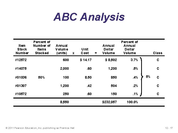
ABC Analysis Item Stock Number Percent of Number of Items Stocked Annual Volume (units) x Unit Cost = Annual Dollar Volume Percent of Annual Dollar Volume Class #12572 600 $ 14. 17 $ 8, 502 3. 7% C #14075 2, 000 . 60 1, 200 . 5% C 100 8. 50 850 . 4% #01307 1, 200 . 42 504 . 2% C #10572 250 . 60 150 . 1% C $232, 057 100. 0% #01036 50% 8, 550 © 2011 Pearson Education, Inc. publishing as Prentice Hall 5% C 12 - 17
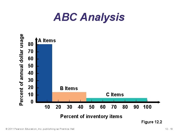
Percent of annual dollar usage ABC Analysis 80 70 60 50 40 30 20 10 0 A Items – – – – B Items – | | – 10 20 30 40 C Items | | 50 60 70 80 | | 90 100 Percent of inventory items Figure 12. 2 © 2011 Pearson Education, Inc. publishing as Prentice Hall 12 - 18
ABC Analysis u Policies employed may include u. More emphasis on supplier development for A items u. Tighter physical inventory control for A items u. More care in forecasting A items © 2011 Pearson Education, Inc. publishing as Prentice Hall 12 - 19
Inventory Record Accuracy &Cycle Counting u Items are counted and records are updated on a periodic basis u Often used with ABC analysis to determine the cycle (frequency of counting) u Eliminates shutdowns and interruptions u Maintains accurate inventory records © 2011 Pearson Education, Inc. publishing as Prentice Hall 12 - 20
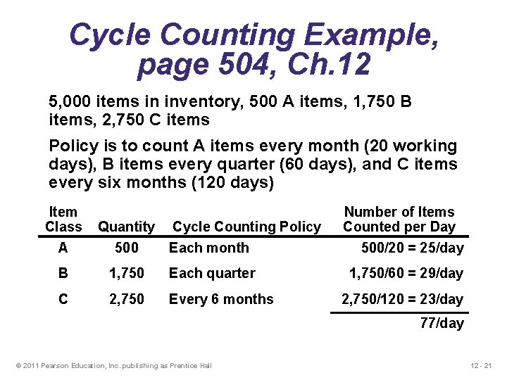
Cycle Counting Example, page 504, Ch. 12 5, 000 items in inventory, 500 A items, 1, 750 B items, 2, 750 C items Policy is to count A items every month (20 working days), B items every quarter (60 days), and C items every six months (120 days) Item Class Quantity A 500 Each month B 1, 750 Each quarter C 2, 750 Every 6 months Cycle Counting Policy Number of Items Counted per Day 500/20 = 25/day 1, 750/60 = 29/day 2, 750/120 = 23/day 77/day © 2011 Pearson Education, Inc. publishing as Prentice Hall 12 - 21
Two Basic Questions to Answer Through Inventory Management 1. How much to order of each material when orders are placed with either outside suppliers or production departments within organizations. 1. When to place the orders. The overall objective of inventory management is to achieve satisfactory levels of customer service while keeping inventory costs within reasonable bounds by answering these two questions. 12 - 22
Inventory Models for Independent Demand Used to determine when and how much to order (Q) 1. Basic Economic Order Quantity (EOQ) 2. Production Order Quantity (POQ) 3. Quantity discount model © 2011 Pearson Education, Inc. publishing as Prentice Hall 12 - 23
Holding, Ordering, and Setup Costs u Holding costs - the costs of holding or “carrying” inventory over time u Ordering costs - the costs of placing an order and receiving goods u Setup costs - cost to prepare a machine or process for manufacturing an order © 2011 Pearson Education, Inc. publishing as Prentice Hall 12 - 24
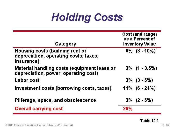
Holding Costs Category Housing costs (building rent or depreciation, operating costs, taxes, insurance) Material handling costs (equipment lease or depreciation, power, operating cost) Labor cost Investment costs (borrowing costs, taxes) Pilferage, space, and obsolescence Overall carrying cost Cost (and range) as a Percent of Inventory Value 6% (3 - 10%) 3% (1 - 3. 5%) 3% (3 - 5%) 11% (6 - 24%) 3% (2 - 5%) 26% Table 12. 1 © 2011 Pearson Education, Inc. publishing as Prentice Hall 12 - 25
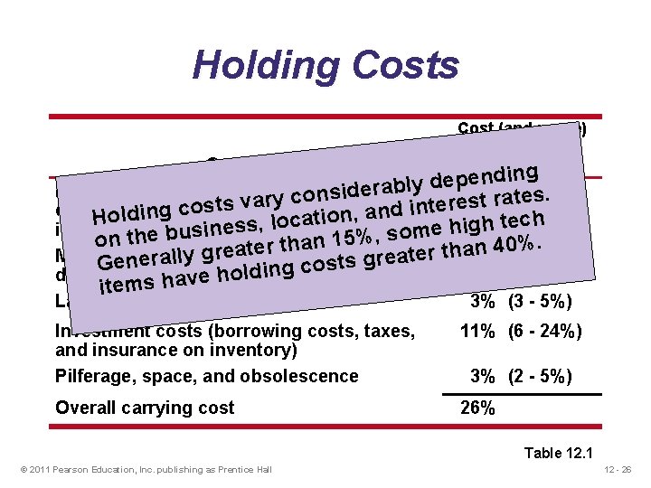
Holding Costs Cost (and range) as a Percent of Inventory Value Category ng i d n e p e d y Housing costs (building rent ornsiderabl 6% a(3 -s 10%). o e c t y r r t a s v e r s t e t s co depreciation, costs, ttaxes, d in n a , n o i Holdingoperating a c ech o t l , h s g i s h e insurance) n e i s m on the bu eater than 15%, so than 40%. r r gcosts e Material handling (equipment lease or 3% (1 - 3. 5%) t y l a l e a r r e g n s e t s G o c ding cost) l o depreciation, power, operating h e v a h items Labor cost 3% (3 - 5%) Investment costs (borrowing costs, taxes, and insurance on inventory) Pilferage, space, and obsolescence 11% (6 - 24%) Overall carrying cost 26% 3% (2 - 5%) Table 12. 1 © 2011 Pearson Education, Inc. publishing as Prentice Hall 12 - 26
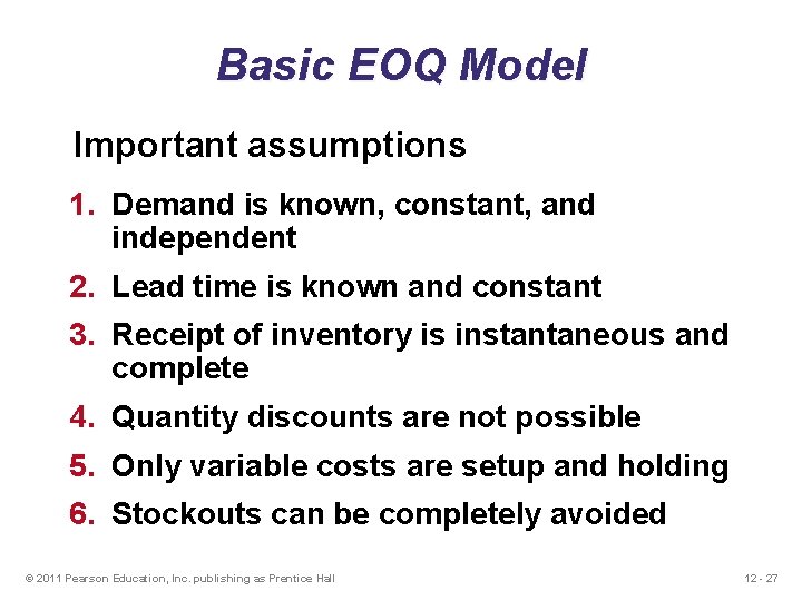
Basic EOQ Model Important assumptions 1. Demand is known, constant, and independent 2. Lead time is known and constant 3. Receipt of inventory is instantaneous and complete 4. Quantity discounts are not possible 5. Only variable costs are setup and holding 6. Stockouts can be completely avoided © 2011 Pearson Education, Inc. publishing as Prentice Hall 12 - 27
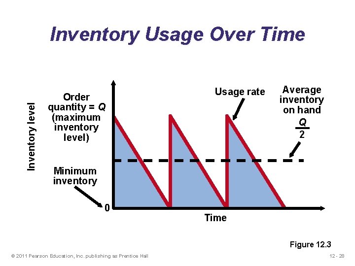
Inventory level Inventory Usage Over Time Order quantity = Q (maximum inventory level) Usage rate Average inventory on hand Q 2 Minimum inventory 0 Time Figure 12. 3 © 2011 Pearson Education, Inc. publishing as Prentice Hall 12 - 28

Minimizing Costs Objective is to minimize total costs Total cost of holding and setup (order) Annual cost Minimum total cost Table 12. 4(c) © 2011 Pearson Education, Inc. publishing as Prentice Hall Holding cost Setup (or order) cost Optimal order quantity (Q*) Order quantity 12 - 29
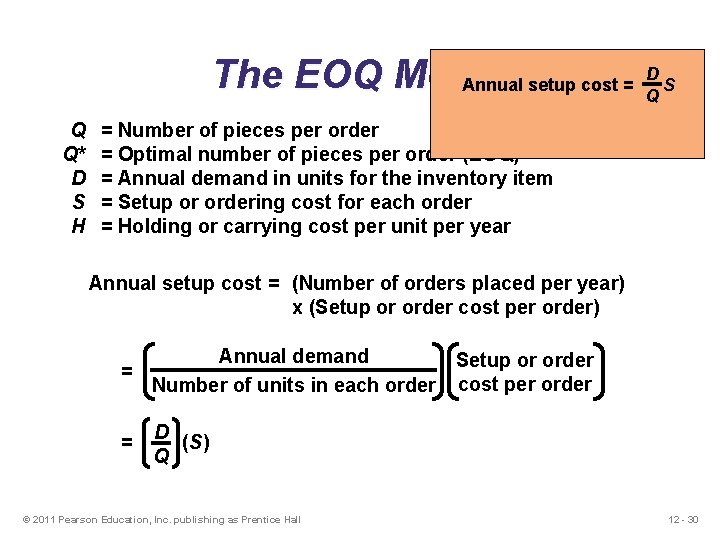
D The EOQ Model Annual setup cost = S Q Q Q* D S H = Number of pieces per order = Optimal number of pieces per order (EOQ) = Annual demand in units for the inventory item = Setup or ordering cost for each order = Holding or carrying cost per unit per year Annual setup cost = (Number of orders placed per year) x (Setup or order cost per order) Annual demand Setup or order = Number of units in each order cost per order = D (S) Q © 2011 Pearson Education, Inc. publishing as Prentice Hall 12 - 30
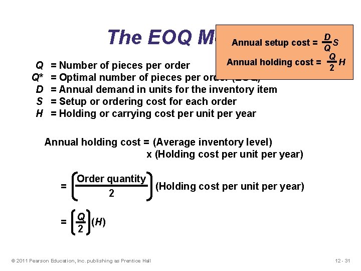
D The EOQ Model Annual setup cost = S Q Q Q* D S H Annual holding cost = = Number of pieces per order = Optimal number of pieces per order (EOQ) = Annual demand in units for the inventory item = Setup or ordering cost for each order = Holding or carrying cost per unit per year Q H 2 Annual holding cost = (Average inventory level) x (Holding cost per unit per year) = Order quantity (Holding cost per unit per year) 2 = Q (H) 2 © 2011 Pearson Education, Inc. publishing as Prentice Hall 12 - 31
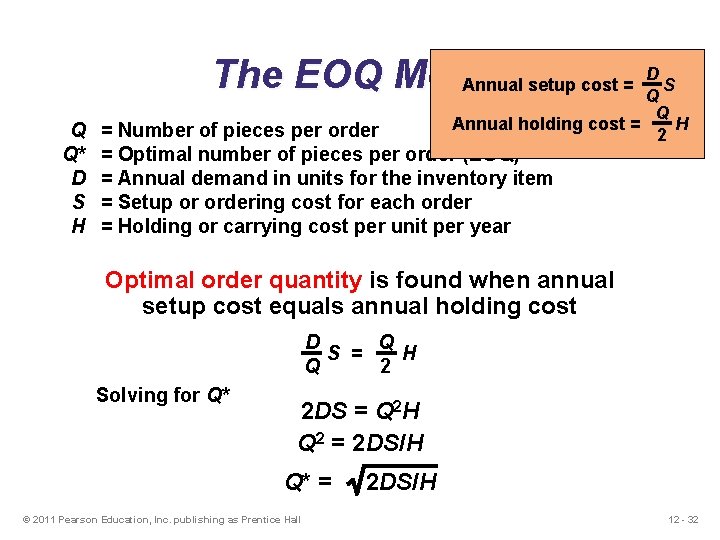
D The EOQ Model Annual setup cost = S Q Q Q* D S H Annual holding cost = = Number of pieces per order = Optimal number of pieces per order (EOQ) = Annual demand in units for the inventory item = Setup or ordering cost for each order = Holding or carrying cost per unit per year Q H 2 Optimal order quantity is found when annual setup cost equals annual holding cost D Q S = H Q 2 Solving for Q* 2 DS = Q 2 H Q 2 = 2 DS/H Q* = © 2011 Pearson Education, Inc. publishing as Prentice Hall 2 DS/H 12 - 32
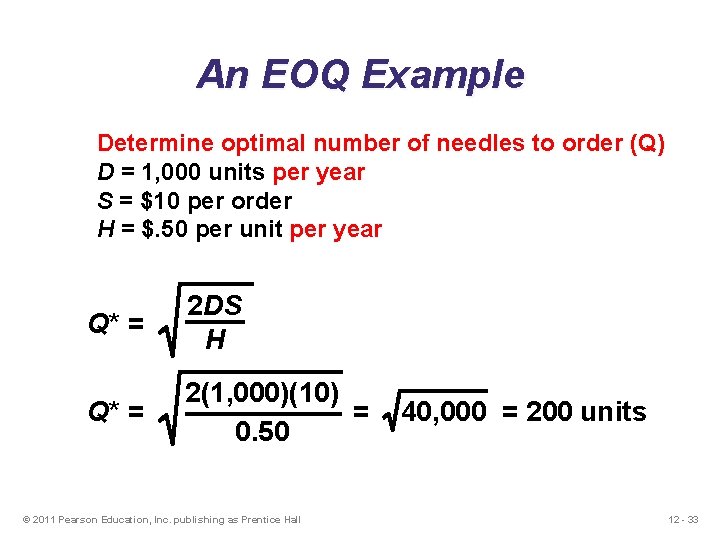
An EOQ Example Determine optimal number of needles to order (Q) D = 1, 000 units per year S = $10 per order H = $. 50 per unit per year Q* = 2 DS H Q* = 2(1, 000)(10) = 0. 50 © 2011 Pearson Education, Inc. publishing as Prentice Hall 40, 000 = 200 units 12 - 33
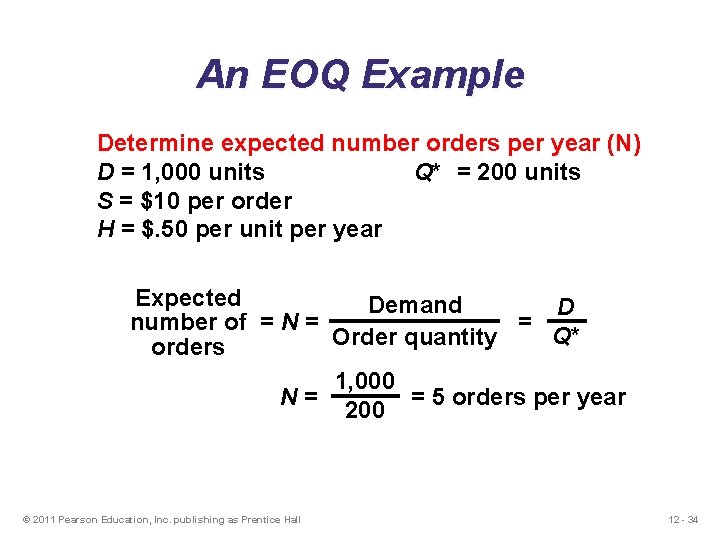
An EOQ Example Determine expected number orders per year (N) D = 1, 000 units Q* = 200 units S = $10 per order H = $. 50 per unit per year Expected Demand D number of = N = = Q* Order quantity orders 1, 000 N= = 5 orders per year 200 © 2011 Pearson Education, Inc. publishing as Prentice Hall 12 - 34
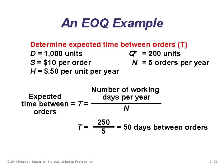
An EOQ Example Determine expected time between orders (T) D = 1, 000 units Q* = 200 units S = $10 per order N = 5 orders per year H = $. 50 per unit per year Expected time between = T = orders Number of working days per year T= © 2011 Pearson Education, Inc. publishing as Prentice Hall N 250 = 50 days between orders 5 12 - 35
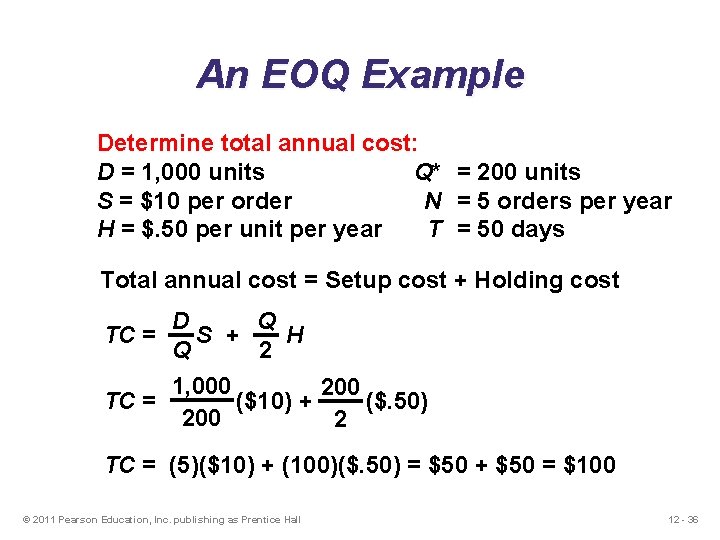
An EOQ Example Determine total annual cost: D = 1, 000 units Q* = 200 units S = $10 per order N = 5 orders per year H = $. 50 per unit per year T = 50 days Total annual cost = Setup cost + Holding cost TC = Q D S + H 2 Q 1, 000 200 TC = ($10) + ($. 50) 200 2 TC = (5)($10) + (100)($. 50) = $50 + $50 = $100 © 2011 Pearson Education, Inc. publishing as Prentice Hall 12 - 36
Robust Model u The EOQ model is robust u It works even if all parameters and assumptions are not met Because the total cost curve is relatively flat in the area of the EOQ © 2011 Pearson Education, Inc. publishing as Prentice Hall 12 - 37
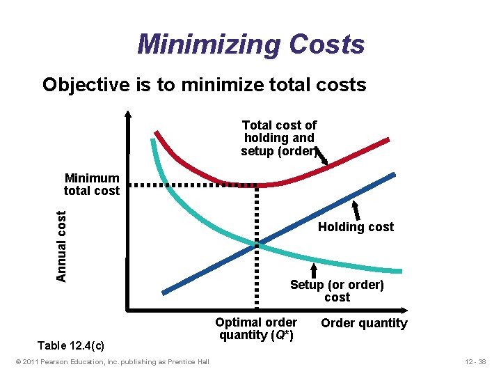
Minimizing Costs Objective is to minimize total costs Total cost of holding and setup (order) Annual cost Minimum total cost Table 12. 4(c) © 2011 Pearson Education, Inc. publishing as Prentice Hall Holding cost Setup (or order) cost Optimal order quantity (Q*) Order quantity 12 - 38
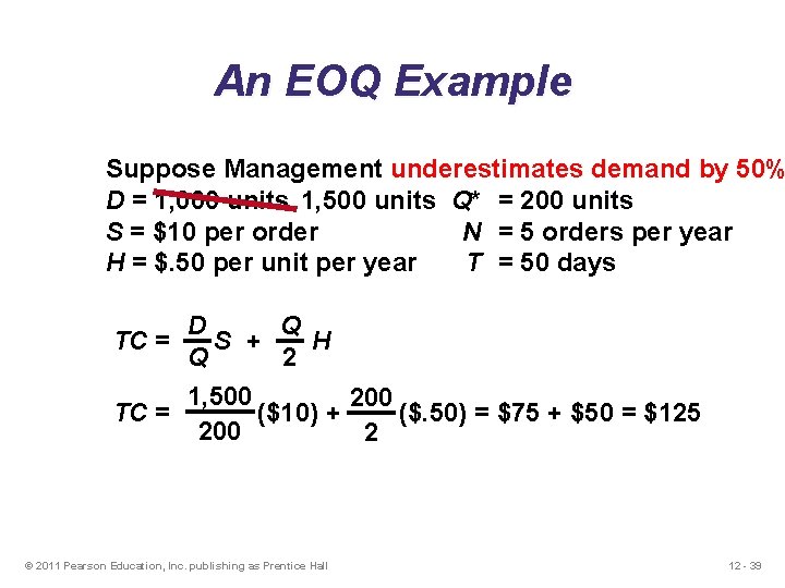
An EOQ Example Suppose Management underestimates demand by 50% D = 1, 000 units 1, 500 units Q* = 200 units S = $10 per order N = 5 orders per year H = $. 50 per unit per year T = 50 days Q D TC = S + H 2 Q TC = 1, 500 200 ($10) + ($. 50) = $75 + $50 = $125 200 2 © 2011 Pearson Education, Inc. publishing as Prentice Hall 12 - 39
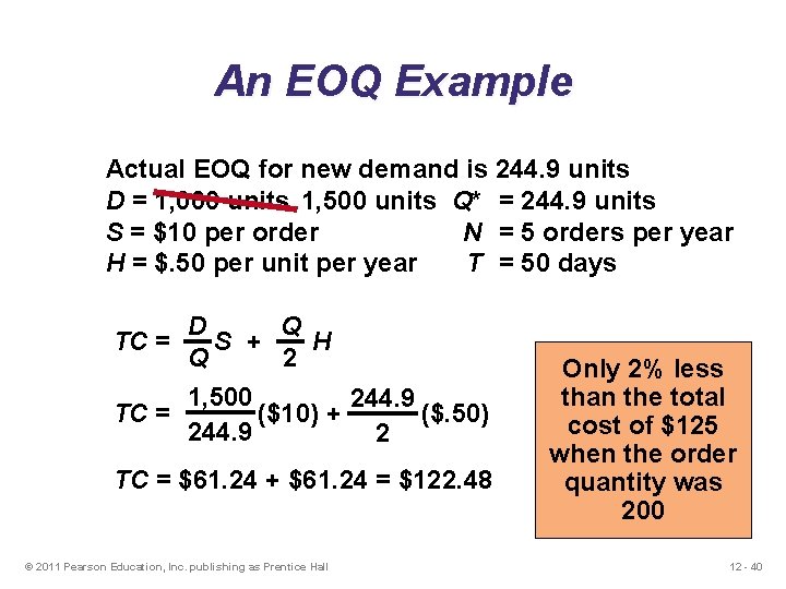
An EOQ Example Actual EOQ for new demand is 244. 9 units D = 1, 000 units 1, 500 units Q* = 244. 9 units S = $10 per order N = 5 orders per year H = $. 50 per unit per year T = 50 days Q D TC = S + H 2 Q TC = 1, 500 244. 9 ($10) + ($. 50) 244. 9 2 TC = $61. 24 + $61. 24 = $122. 48 © 2011 Pearson Education, Inc. publishing as Prentice Hall Only 2% less than the total cost of $125 when the order quantity was 200 12 - 40
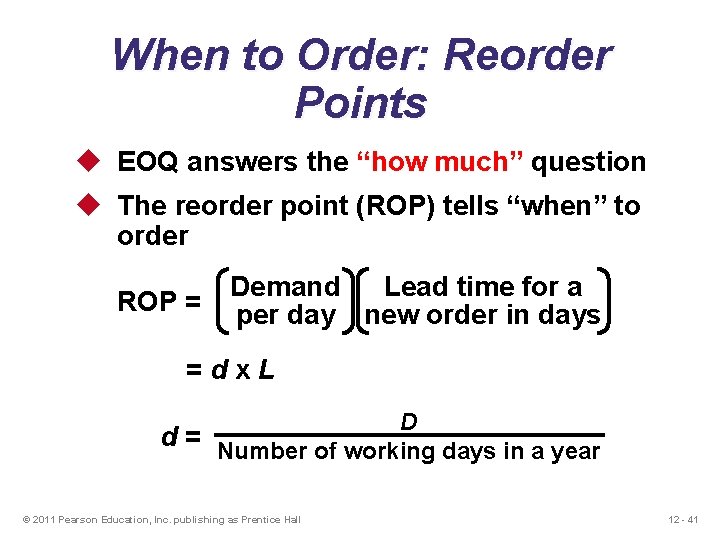
When to Order: Reorder Points u EOQ answers the “how much” question u The reorder point (ROP) tells “when” to order ROP = Lead time for a Demand per day new order in days =dx. L D d = Number of working days in a year © 2011 Pearson Education, Inc. publishing as Prentice Hall 12 - 41
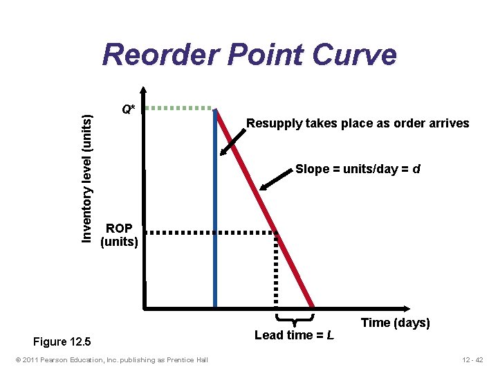
Inventory level (units) Reorder Point Curve Q* Resupply takes place as order arrives Slope = units/day = d ROP (units) Figure 12. 5 © 2011 Pearson Education, Inc. publishing as Prentice Hall Lead time = L Time (days) 12 - 42
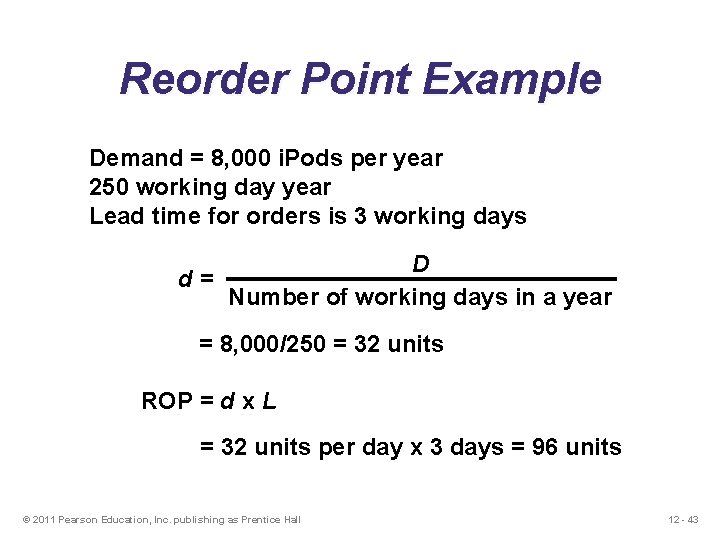
Reorder Point Example Demand = 8, 000 i. Pods per year 250 working day year Lead time for orders is 3 working days D d= Number of working days in a year = 8, 000/250 = 32 units ROP = d x L = 32 units per day x 3 days = 96 units © 2011 Pearson Education, Inc. publishing as Prentice Hall 12 - 43
Production Order Quantity (POQ) Model u Used when the third assumption of EOQ model is relaxed: Receipt of inventory is not instantaneous and complete u Used when units are produced and used/or sold simultaneously u Hence, inventory builds up over a period of time after an order is placed © 2011 Pearson Education, Inc. publishing as Prentice Hall 12 - 44
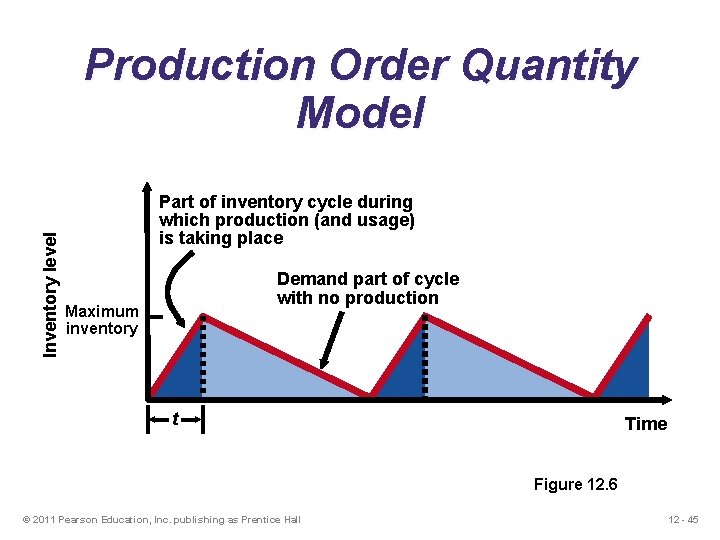
Inventory level Production Order Quantity Model Part of inventory cycle during which production (and usage) is taking place Demand part of cycle with no production Maximum inventory t Time Figure 12. 6 © 2011 Pearson Education, Inc. publishing as Prentice Hall 12 - 45
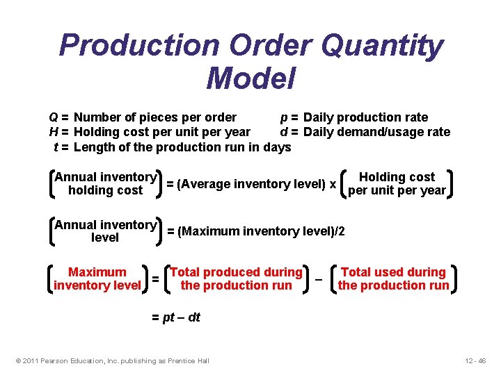
Production Order Quantity Model Q = Number of pieces per order p = Daily production rate H = Holding cost per unit per year d = Daily demand/usage rate t = Length of the production run in days Holding cost Annual inventory = (Average inventory level) x per unit per year holding cost Annual inventory = (Maximum inventory level)/2 level Total produced during Maximum = – the production run inventory level Total used during the production run = pt – dt © 2011 Pearson Education, Inc. publishing as Prentice Hall 12 - 46
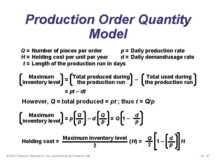
Production Order Quantity Model Q = Number of pieces per order p = Daily production rate H = Holding cost per unit per year d = Daily demand/usage rate t = Length of the production run in days Total produced during Maximum = – the production run inventory level Total used during the production run = pt – dt However, Q = total produced = pt ; thus t = Q/p Q Maximum = p inventory level p Holding cost = –d Q p =Q 1– d p Maximum inventory level (H) = 2 © 2011 Pearson Education, Inc. publishing as Prentice Hall Q d 1– 2 p H 12 - 47

Production Order Quantity Model Q = Number of pieces per order H = Holding cost per unit per year D = Annual demand p = Daily production rate d = Daily demand/usage rate Setup cost = (D/Q)S Holding cost = 1 2 HQ[1 - (d/p)] 1 (D/Q)S = 2 HQ[1 - (d/p)] 2 DS 2 Q = H[1 - (d/p)] Q*p = © 2011 Pearson Education, Inc. publishing as Prentice Hall 2 DS H[1 - (d/p)] 12 - 48
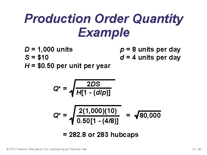
Production Order Quantity Example D = 1, 000 units S = $10 H = $0. 50 per unit per year Q* = 2 DS H[1 - (d/p)] Q* = 2(1, 000)(10) 0. 50[1 - (4/8)] p = 8 units per day d = 4 units per day = 80, 000 = 282. 8 or 283 hubcaps © 2011 Pearson Education, Inc. publishing as Prentice Hall 12 - 49
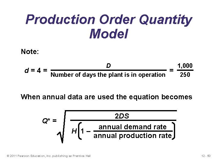
Production Order Quantity Model Note: d=4= D Number of days the plant is in operation = 1, 000 250 When annual data are used the equation becomes Q* = 2 DS annual demand rate H 1– annual production rate © 2011 Pearson Education, Inc. publishing as Prentice Hall 12 - 50
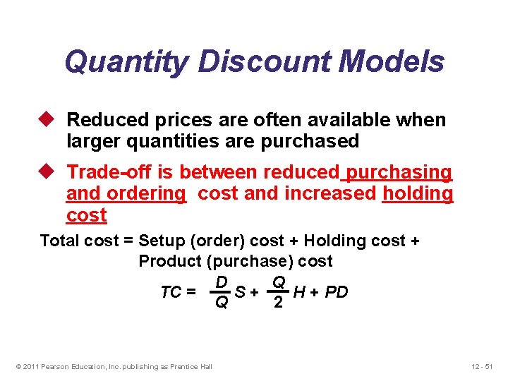
Quantity Discount Models u Reduced prices are often available when larger quantities are purchased u Trade-off is between reduced purchasing and ordering cost and increased holding cost Total cost = Setup (order) cost + Holding cost + Product (purchase) cost D Q TC = S+ H + PD Q 2 © 2011 Pearson Education, Inc. publishing as Prentice Hall 12 - 51
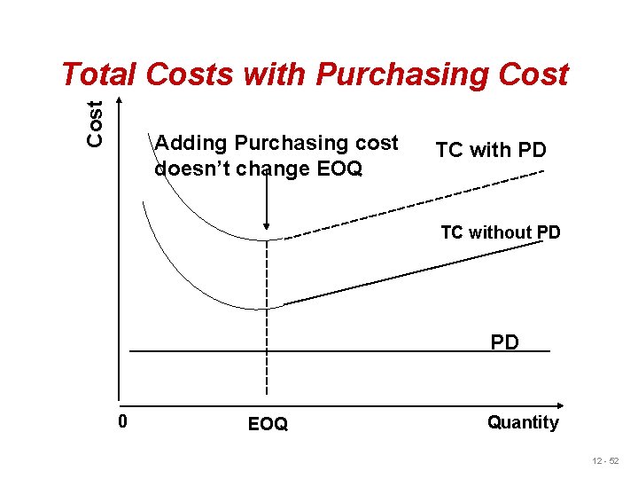
Cost Total Costs with Purchasing Cost Adding Purchasing cost doesn’t change EOQ TC with PD TC without PD PD 0 EOQ Quantity 12 - 52
Quantity Discount Models u There are two general cases of quantity discount models: 1. Carrying costs are constant (e. g. $2 per unit). 2. Carrying costs are stated as a percentage off purchase price (20% of unit price) © 2011 Pearson Education, Inc. publishing as Prentice Hall 12 - 53
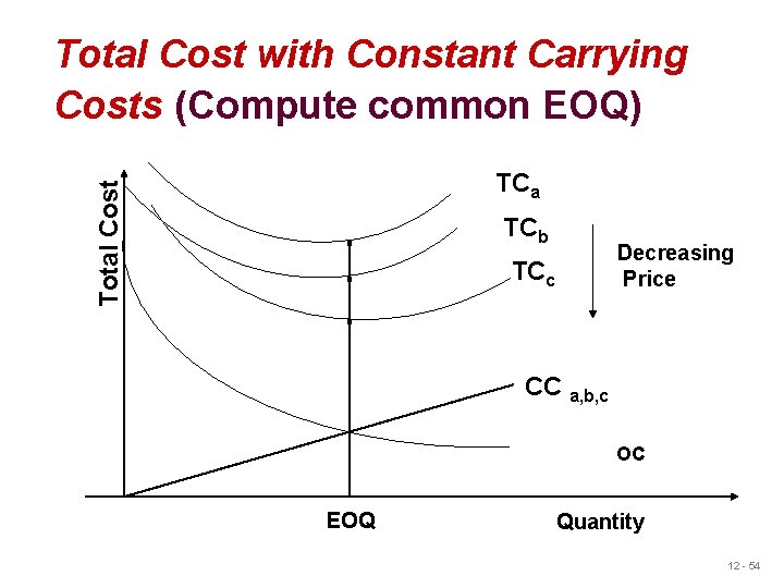
Total Cost with Constant Carrying Costs (Compute common EOQ) Total Cost TCa TCb Decreasing Price TCc CC a, b, c OC EOQ Quantity 12 - 54
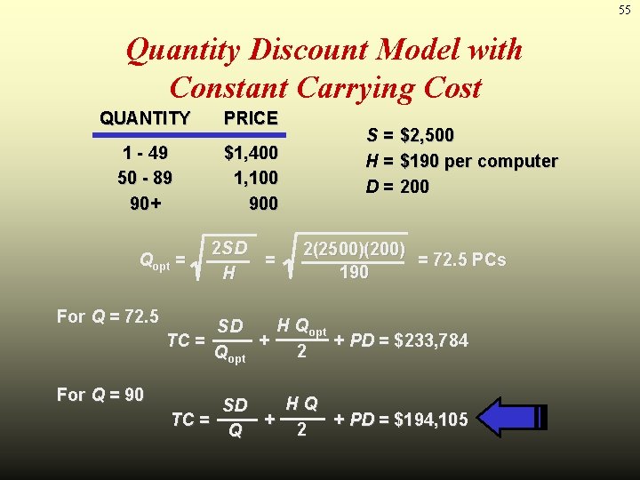
55 Quantity Discount Model with Constant Carrying Cost QUANTITY PRICE 1 - 49 50 - 89 90+ $1, 400 1, 100 900 Qopt = For Q = 72. 5 For Q = 90 2 S D = H S= H= D= $2, 500 $190 per computer 200 2(2500)(200) = 72. 5 PCs 190 H Qopt SD TC = + + PD = $233, 784 2 Qopt HQ SD TC = + + PD = $194, 105 2 Q
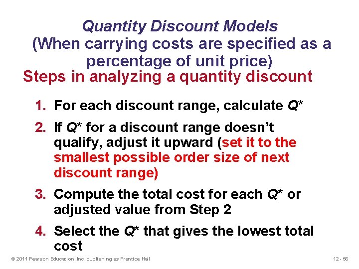
Quantity Discount Models (When carrying costs are specified as a percentage of unit price) Steps in analyzing a quantity discount 1. For each discount range, calculate Q* 2. If Q* for a discount range doesn’t qualify, adjust it upward (set it to the smallest possible order size of next discount range) 3. Compute the total cost for each Q* or adjusted value from Step 2 4. Select the Q* that gives the lowest total cost © 2011 Pearson Education, Inc. publishing as Prentice Hall 12 - 56

Quantity Discount Models A typical quantity discount schedule, Inventory Carrying cost is 20% of unit price Discount Number Discount Quantity Discount (%) Discount Price (P) 1 0 to 999 no discount $5. 00 2 1, 000 to 1, 999 4 $4. 80 3 2, 000 and over 5 $4. 75 Table 12. 2 © 2011 Pearson Education, Inc. publishing as Prentice Hall 12 - 57
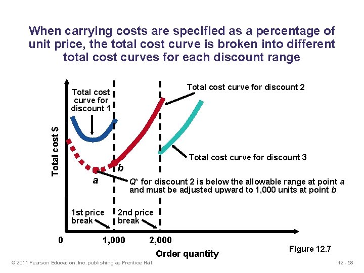
When carrying costs are specified as a percentage of unit price, the total cost curve is broken into different total cost curves for each discount range Total cost curve for discount 2 Total cost $ Total cost curve for discount 1 Total cost curve for discount 3 b a Q* for discount 2 is below the allowable range at point a and must be adjusted upward to 1, 000 units at point b 1 st price break 0 2 nd price break 1, 000 2, 000 Order quantity © 2011 Pearson Education, Inc. publishing as Prentice Hall Figure 12. 7 12 - 58

Quantity Discount Example Calculate Q* for every discount Q* = 2 DS IP Q 1* = 2(5, 000)(49) = 700 cars/order (. 2)(5. 00) Q 2* = 2(5, 000)(49) = 714 cars/order (. 2)(4. 80) Q 3* = 2(5, 000)(49) = 718 cars/order (. 2)(4. 75) © 2011 Pearson Education, Inc. publishing as Prentice Hall 12 - 59
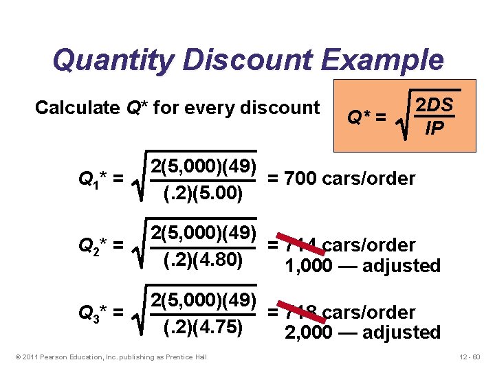
Quantity Discount Example Calculate Q* for every discount Q* = 2 DS IP Q 1* = 2(5, 000)(49) = 700 cars/order (. 2)(5. 00) Q 2* = 2(5, 000)(49) = 714 cars/order (. 2)(4. 80) 1, 000 — adjusted Q 3* = 2(5, 000)(49) = 718 cars/order (. 2)(4. 75) 2, 000 — adjusted © 2011 Pearson Education, Inc. publishing as Prentice Hall 12 - 60
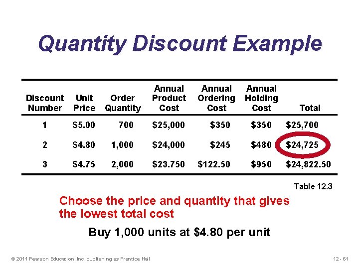
Quantity Discount Example Order Quantity Annual Product Cost Annual Ordering Cost Annual Holding Cost Discount Number Unit Price 1 $5. 00 700 $25, 000 $350 $25, 700 2 $4. 80 1, 000 $245 $480 $24, 725 3 $4. 75 2, 000 $23. 750 $122. 50 $950 $24, 822. 50 Total Table 12. 3 Choose the price and quantity that gives the lowest total cost Buy 1, 000 units at $4. 80 per unit © 2011 Pearson Education, Inc. publishing as Prentice Hall 12 - 61

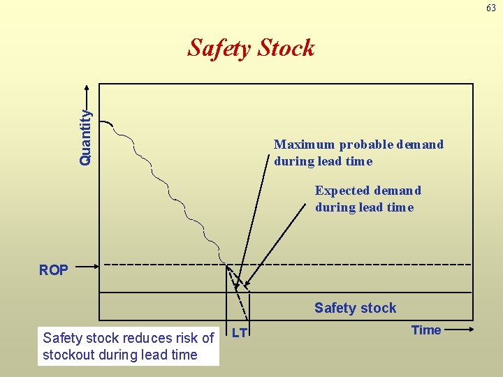
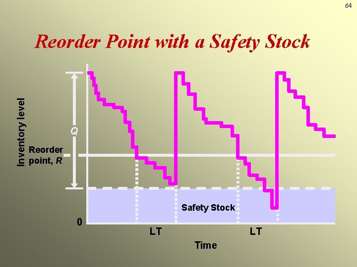
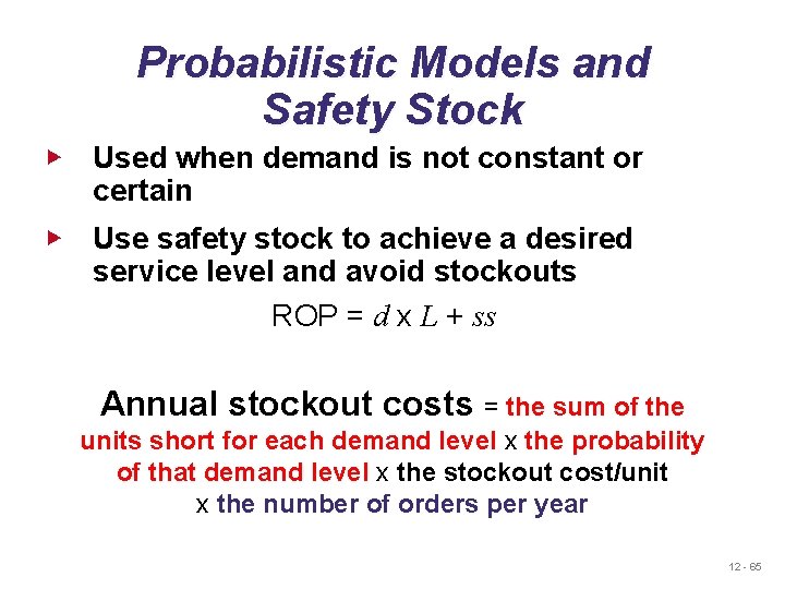
Probabilistic Models Ø Answer how much & when to order Ø Allow demand lead time to vary Ø Consider service level & safety stock § Service level = 1 - Probability of stockout § Higher service level means more safety stock § More safety stock means higher ROP 12 - 62
63 Quantity Safety Stock Maximum probable demand during lead time Expected demand during lead time ROP Safety stock reduces risk of stockout during lead time LT Time
64 Inventory level Reorder Point with a Safety Stock Q Reorder point, R Safety Stock 0 LT LT Time
Probabilistic Models and Safety Stock ▶ Used when demand is not constant or certain ▶ Use safety stock to achieve a desired service level and avoid stockouts ROP = d x L + ss Annual stockout costs = the sum of the units short for each demand level x the probability of that demand level x the stockout cost/unit x the number of orders per year 12 - 65
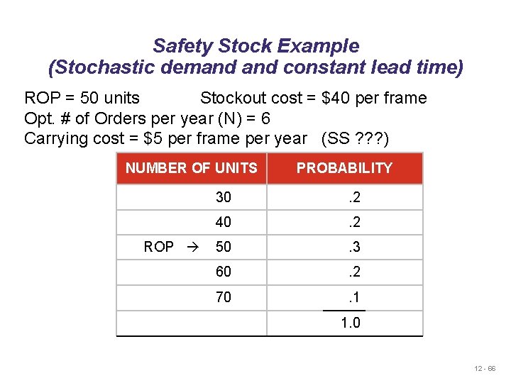
Safety Stock Example (Stochastic demand constant lead time) ROP = 50 units Stockout cost = $40 per frame Opt. # of Orders per year (N) = 6 Carrying cost = $5 per frame per year (SS ? ? ? ) NUMBER OF UNITS ROP PROBABILITY 30 . 2 40 . 2 50 . 3 60 . 2 70 . 1 1. 0 12 - 66
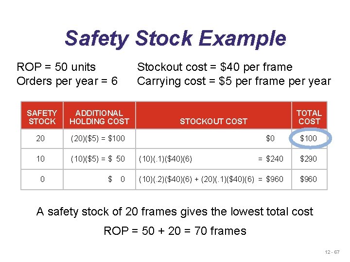
Safety Stock Example ROP = 50 units Orders per year = 6 Stockout cost = $40 per frame Carrying cost = $5 per frame per year SAFETY STOCK ADDITIONAL HOLDING COST 20 (20)($5) = $100 10 (10)($5) = $ 50 0 $ 0 TOTAL COST STOCKOUT COST $0 $100 = $240 $290 (10)(. 2)($40)(6) + (20)(. 1)($40)(6) = $960 (10)(. 1)($40)(6) A safety stock of 20 frames gives the lowest total cost ROP = 50 + 20 = 70 frames 12 - 67
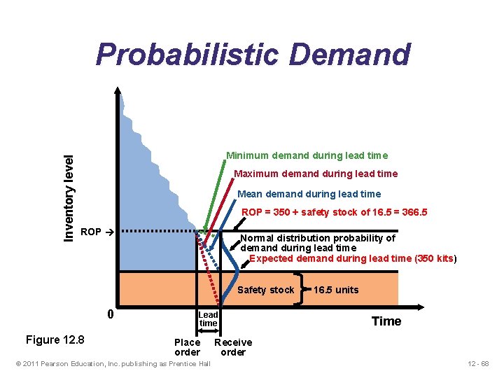
Inventory level Probabilistic Demand Minimum demand during lead time Maximum demand during lead time Mean demand during lead time ROP = 350 + safety stock of 16. 5 = 366. 5 ROP Normal distribution probability of demand during lead time Expected demand during lead time (350 kits) Safety stock 0 Figure 12. 8 Lead time Place order © 2011 Pearson Education, Inc. publishing as Prentice Hall 16. 5 units Time Receive order 12 - 68
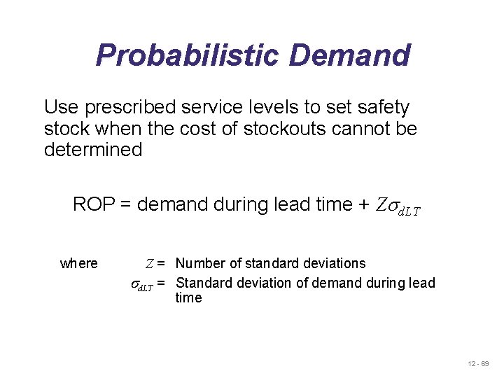
Probabilistic Demand Use prescribed service levels to set safety stock when the cost of stockouts cannot be determined ROP = demand during lead time + Zsd. LT where Z = Number of standard deviations sd. LT = Standard deviation of demand during lead time 12 - 69
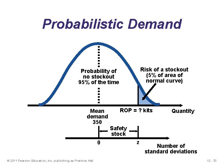
Probabilistic Demand Risk of a stockout (5% of area of normal curve) Probability of no stockout 95% of the time Mean demand 350 0 © 2011 Pearson Education, Inc. publishing as Prentice Hall ROP = ? kits Quantity Safety stock z Number of standard deviations 12 - 70
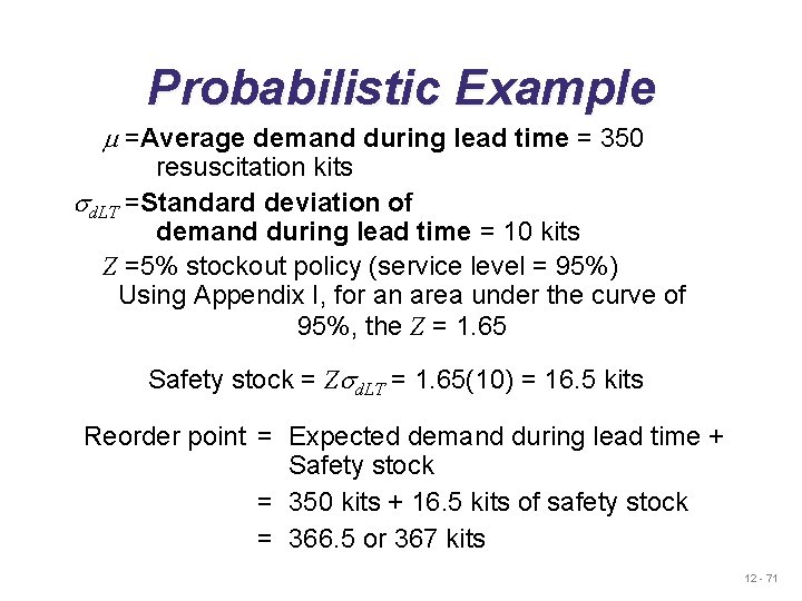
Probabilistic Example m =Average demand during lead time = 350 resuscitation kits sd. LT =Standard deviation of demand during lead time = 10 kits Z =5% stockout policy (service level = 95%) Using Appendix I, for an area under the curve of 95%, the Z = 1. 65 Safety stock = Zsd. LT = 1. 65(10) = 16. 5 kits Reorder point = Expected demand during lead time + Safety stock = 350 kits + 16. 5 kits of safety stock = 366. 5 or 367 kits 12 - 71
Get the probability from standard normal table u z denotes a standard normal random variable u Standard normal curve is symmetric about the origin 0 u Draw a graph 12 - 72

Get the probability from standard normal table u z denotes a standard normal random variable u Standard normal curve is symmetric about the origin 0 u Draw a graph 12 - 73

From non-standard normal to standard normal u X is a normal random variable with mean μ, and standard deviation σ u Set Z=(X–μ)/σ Z=standard unit or z-score of X Then Z has a standard normal distribution and 12 - 74
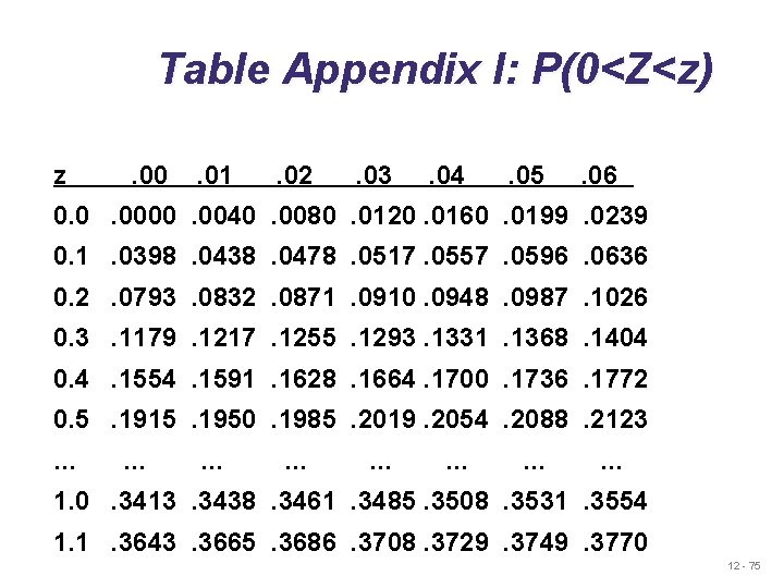
Table Appendix I: P(0<Z<z) z . 00 . 01 . 02 . 03 . 04 . 05 . 06 0. 0. 0000. 0040. 0080. 0120. 0160. 0199. 0239 0. 1. 0398. 0438. 0478. 0517. 0557. 0596. 0636 0. 2. 0793. 0832. 0871. 0910. 0948. 0987. 1026 0. 3. 1179. 1217. 1255. 1293. 1331. 1368. 1404 0. 4. 1554. 1591. 1628. 1664. 1700. 1736. 1772 0. 5. 1915. 1950. 1985. 2019. 2054. 2088. 2123 … … … … 1. 0. 3413. 3438. 3461. 3485. 3508. 3531. 3554 1. 1. 3643. 3665. 3686. 3708. 3729. 3749. 3770 12 - 75
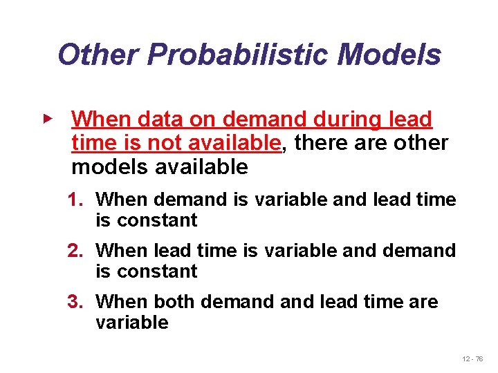
Other Probabilistic Models ▶ When data on demand during lead time is not available, there are other models available 1. When demand is variable and lead time is constant 2. When lead time is variable and demand is constant 3. When both demand lead time are variable 12 - 76
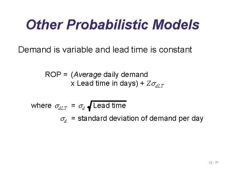
Other Probabilistic Models Demand is variable and lead time is constant ROP = (Average daily demand x Lead time in days) + Zsd. LT where sd. LT = sd Lead time sd = standard deviation of demand per day 12 - 77
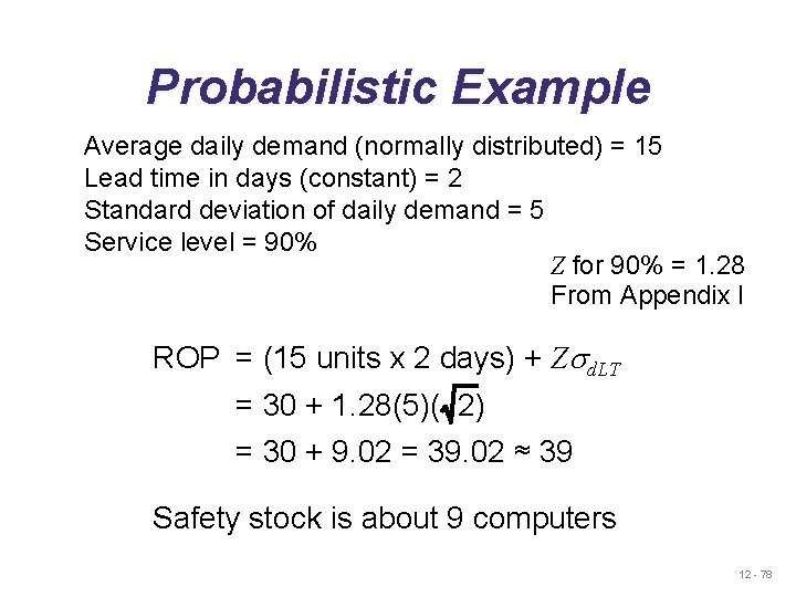
Probabilistic Example Average daily demand (normally distributed) = 15 Lead time in days (constant) = 2 Standard deviation of daily demand = 5 Service level = 90% Z for 90% = 1. 28 From Appendix I ROP = (15 units x 2 days) + Zsd. LT = 30 + 1. 28(5)( 2) = 30 + 9. 02 = 39. 02 ≈ 39 Safety stock is about 9 computers 12 - 78
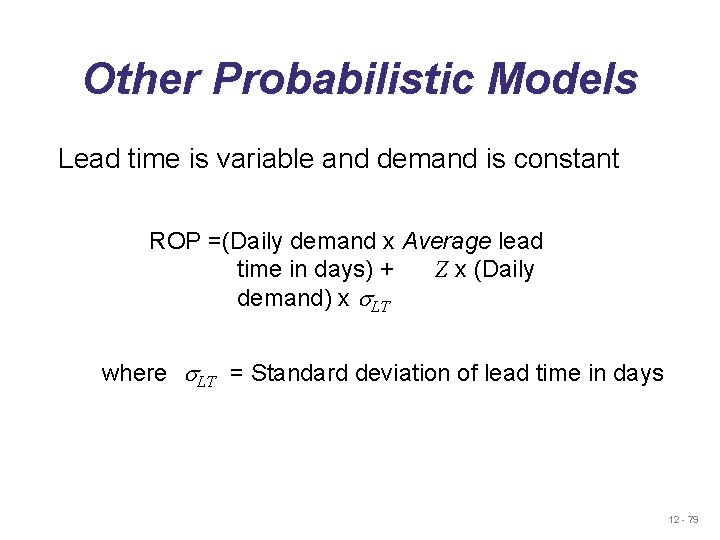
Other Probabilistic Models Lead time is variable and demand is constant ROP =(Daily demand x Average lead time in days) + Z x (Daily demand) x s. LT where s. LT = Standard deviation of lead time in days 12 - 79
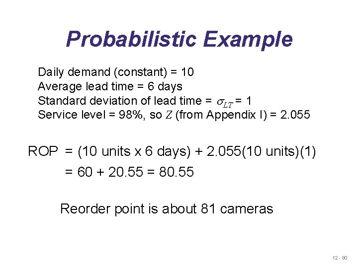
Probabilistic Example Daily demand (constant) = 10 Average lead time = 6 days Standard deviation of lead time = s. LT = 1 Service level = 98%, so Z (from Appendix I) = 2. 055 ROP = (10 units x 6 days) + 2. 055(10 units)(1) = 60 + 20. 55 = 80. 55 Reorder point is about 81 cameras 12 - 80
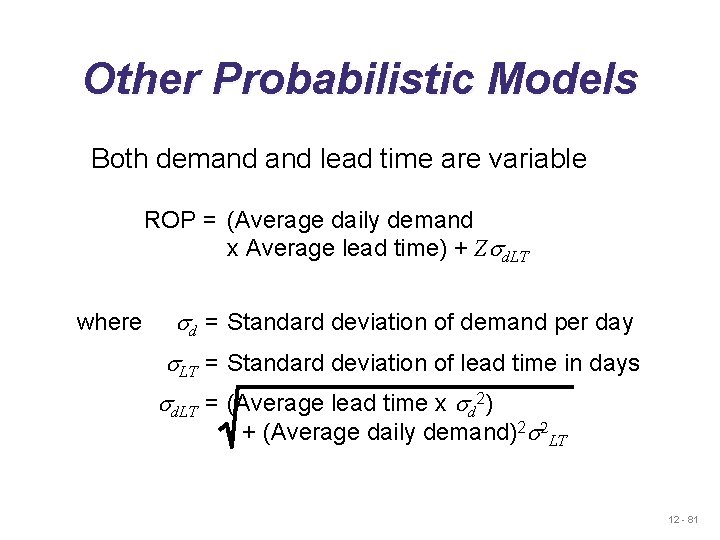
Other Probabilistic Models Both demand lead time are variable ROP = (Average daily demand x Average lead time) + Zsd. LT where sd = Standard deviation of demand per day s. LT = Standard deviation of lead time in days sd. LT = (Average lead time x sd 2) + (Average daily demand)2 s 2 LT 12 - 81
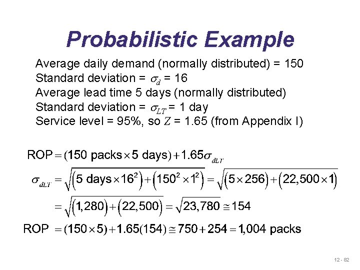
Probabilistic Example Average daily demand (normally distributed) = 150 Standard deviation = sd = 16 Average lead time 5 days (normally distributed) Standard deviation = s. LT = 1 day Service level = 95%, so Z = 1. 65 (from Appendix I) 12 - 82
Single-Period Inventory Model Used to handle ordering of perishables (fresh fruits, flowers) and other items with limited useful lives (newspapers, spare parts for specialized equipment). 12 - 83
Single-Period Inventory Model u In a single-period model, items are received in the beginning of a period and sold during the same period. The unsold items are not carried over to the next period. u The unsold items may be a total waste, or sold at a reduced price, or returned to the producer at some price less than the original purchase price. u The revenue generated by the unsold items is called the salvage value. 12 - 84
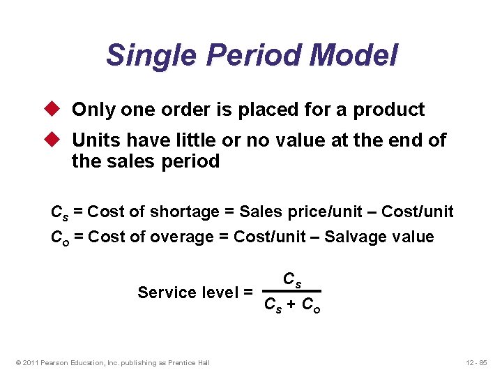
Single Period Model u Only one order is placed for a product u Units have little or no value at the end of the sales period Cs = Cost of shortage = Sales price/unit – Cost/unit Co = Cost of overage = Cost/unit – Salvage value Cs Service level = Cs + Co © 2011 Pearson Education, Inc. publishing as Prentice Hall 12 - 85
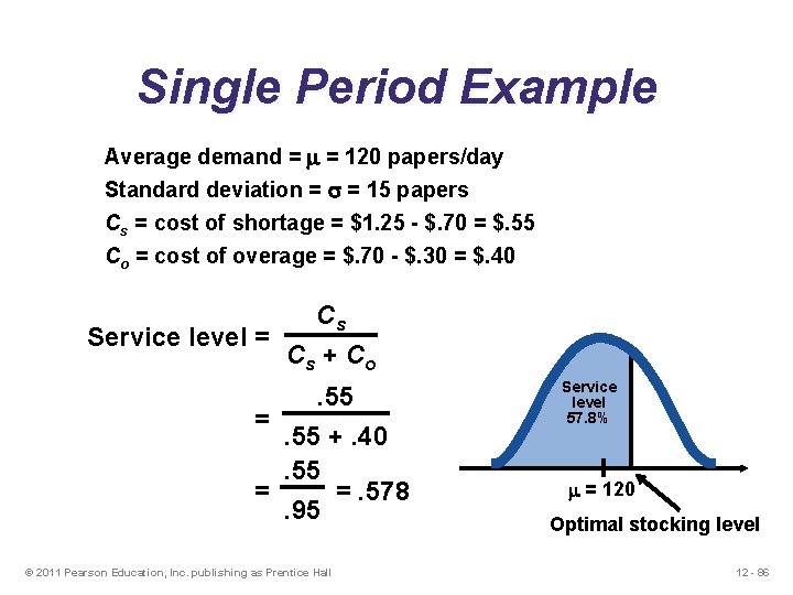
Single Period Example Average demand = = 120 papers/day Standard deviation = = 15 papers Cs = cost of shortage = $1. 25 - $. 70 = $. 55 Co = cost of overage = $. 70 - $. 30 = $. 40 Cs Service level = Cs + Co. 55 =. 55 +. 40. 55 = =. 578. 95 © 2011 Pearson Education, Inc. publishing as Prentice Hall Service level 57. 8% = 120 Optimal stocking level 12 - 86

Single Period Example From Appendix I, for the area. 578, Z . 20 The optimal stocking level = 120 copies + (. 20)( ) = 120 + (. 20)(15) = 120 + 3 = 123 papers The stockout risk = 1 – service level = 1 –. 578 =. 422 = 42. 2% © 2011 Pearson Education, Inc. publishing as Prentice Hall 12 - 87
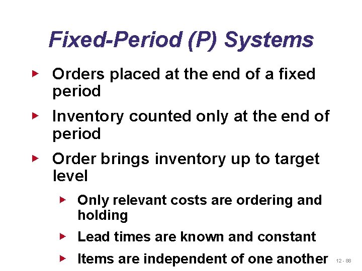
Fixed-Period (P) Systems ▶ Orders placed at the end of a fixed period ▶ Inventory counted only at the end of period ▶ Order brings inventory up to target level ▶ Only relevant costs are ordering and holding ▶ Lead times are known and constant ▶ Items are independent of one another 12 - 88
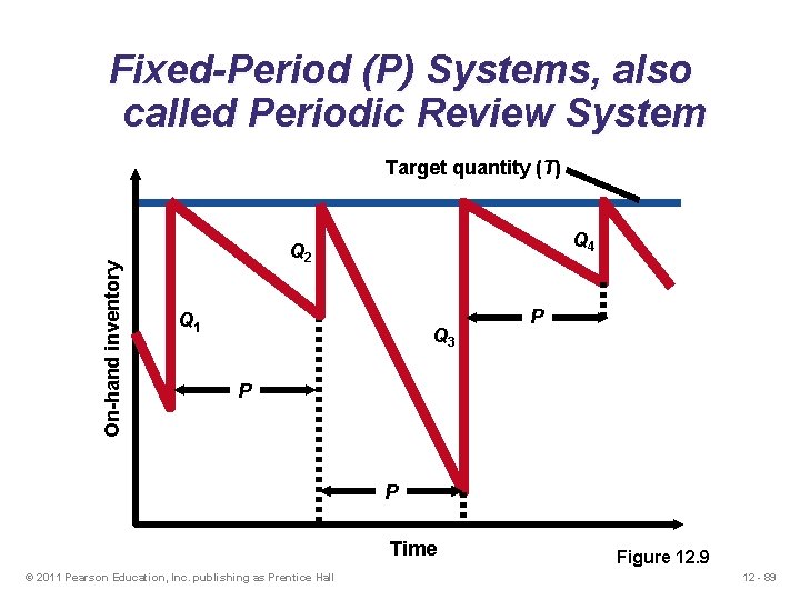
Fixed-Period (P) Systems, also called Periodic Review System On-hand inventory Target quantity (T) Q 4 Q 2 Q 1 Q 3 P P P Time © 2011 Pearson Education, Inc. publishing as Prentice Hall Figure 12. 9 12 - 89
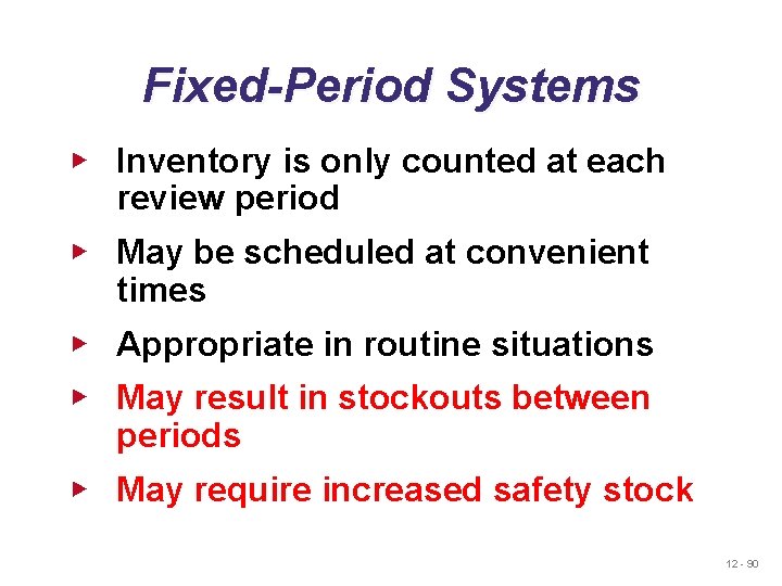
Fixed-Period Systems ▶ Inventory is only counted at each review period ▶ May be scheduled at convenient times ▶ Appropriate in routine situations ▶ May result in stockouts between periods ▶ May require increased safety stock 12 - 90
- Slides: 90