111811 Structure from Motion Computer Vision CS 143

11/18/11 Structure from Motion Computer Vision CS 143, Brown James Hays Many slides adapted from Derek Hoiem, Lana Lazebnik, Silvio Saverese, Steve Seitz, and Martial Hebert

This class: structure from motion • Recap of epipolar geometry – Depth from two views • Affine structure from motion

Recap: Epipoles • Point x in left image corresponds to epipolar line l’ in right image • Epipolar line passes through the epipole (the intersection of the cameras’ baseline with the image plane

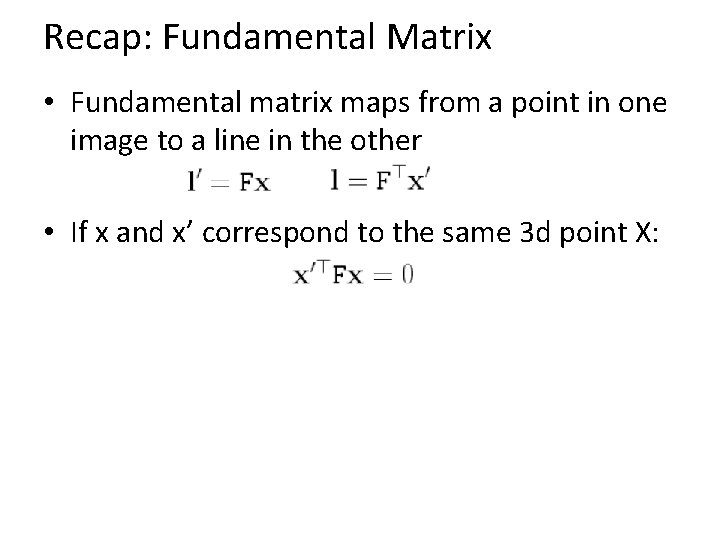
Recap: Fundamental Matrix • Fundamental matrix maps from a point in one image to a line in the other • If x and x’ correspond to the same 3 d point X:

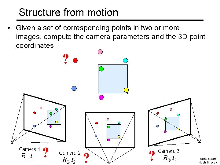
Structure from motion • Given a set of corresponding points in two or more images, compute the camera parameters and the 3 D point coordinates ? Camera 1 R 1, t 1 ? Camera 2 R 2, t 2 ? ? Camera 3 R 3, t 3 Slide credit: Noah Snavely

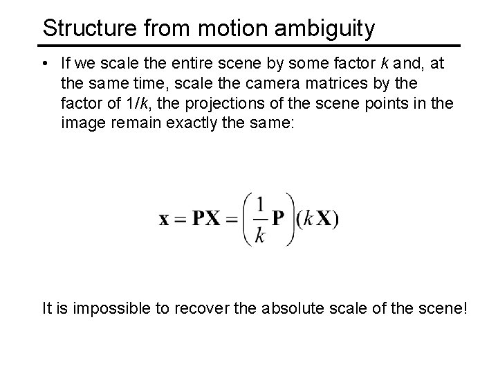
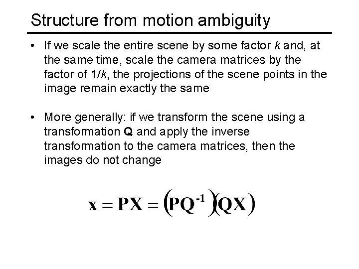
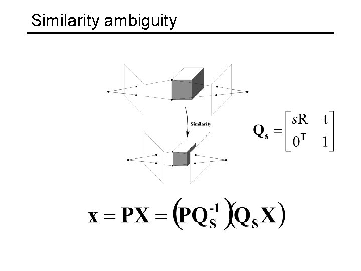
Structure from motion ambiguity • If we scale the entire scene by some factor k and, at the same time, scale the camera matrices by the factor of 1/k, the projections of the scene points in the image remain exactly the same: It is impossible to recover the absolute scale of the scene!

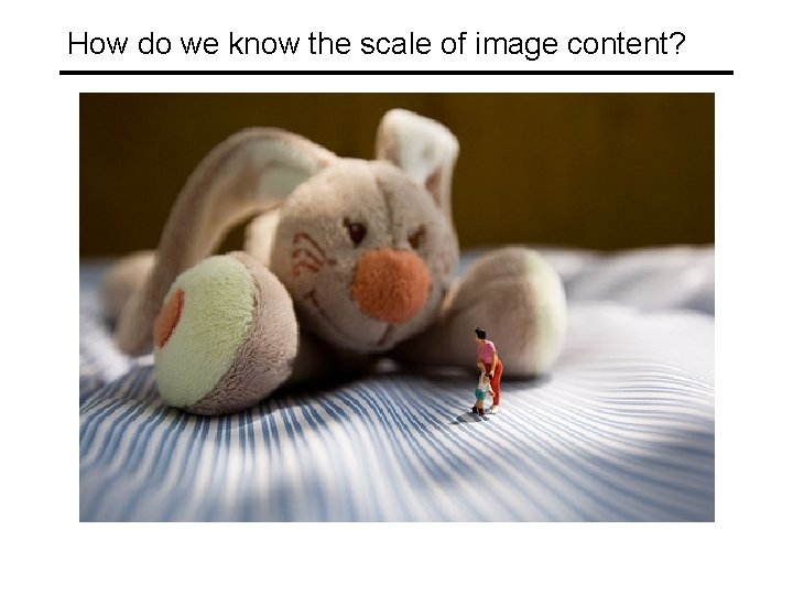
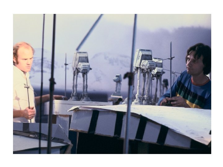
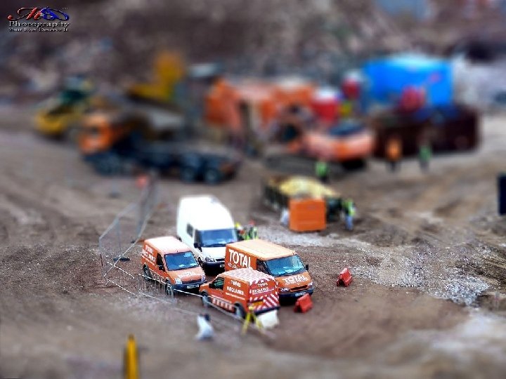
How do we know the scale of image content?

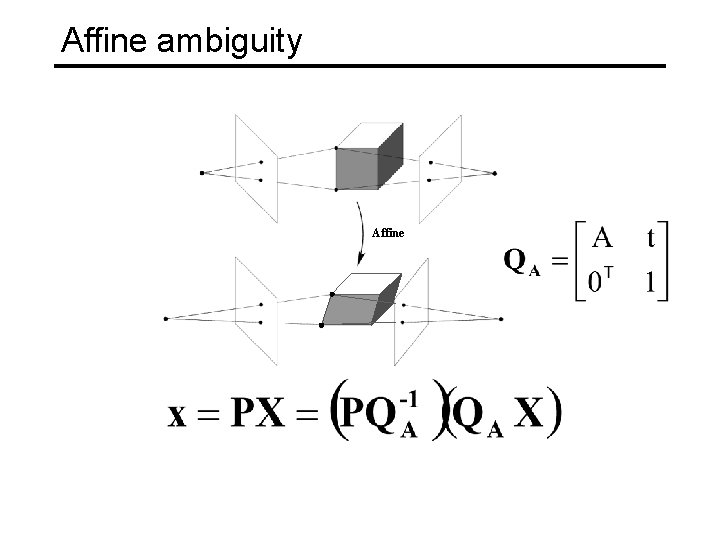
Structure from motion ambiguity • If we scale the entire scene by some factor k and, at the same time, scale the camera matrices by the factor of 1/k, the projections of the scene points in the image remain exactly the same • More generally: if we transform the scene using a transformation Q and apply the inverse transformation to the camera matrices, then the images do not change

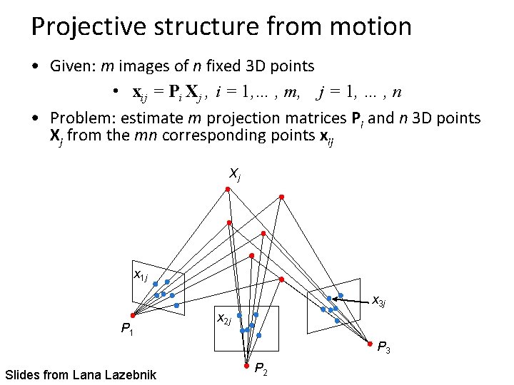
Projective structure from motion • Given: m images of n fixed 3 D points • xij = Pi Xj , i = 1, … , m, j = 1, … , n • Problem: estimate m projection matrices Pi and n 3 D points Xj from the mn corresponding points xij Xj x 1 j x 3 j P 1 x 2 j P 3 Slides from Lana Lazebnik P 2

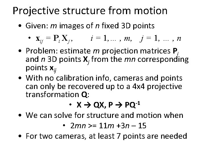
Projective structure from motion • Given: m images of n fixed 3 D points • xij = Pi Xj , i = 1, … , m, j = 1, … , n • Problem: estimate m projection matrices Pi and n 3 D points Xj from the mn corresponding points xij • With no calibration info, cameras and points can only be recovered up to a 4 x 4 projective transformation Q: • X → QX, P → PQ-1 • We can solve for structure and motion when • 2 mn >= 11 m +3 n – 15 • For two cameras, at least 7 points are needed

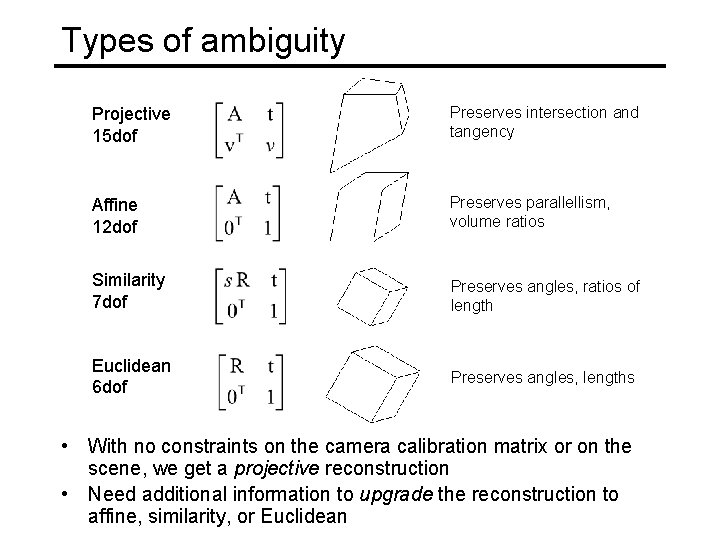
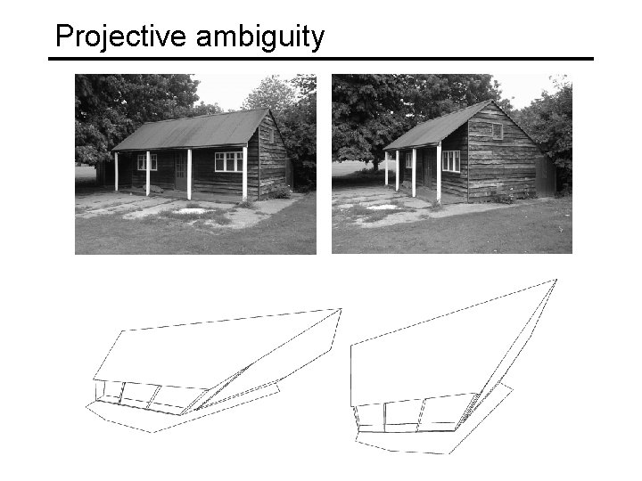
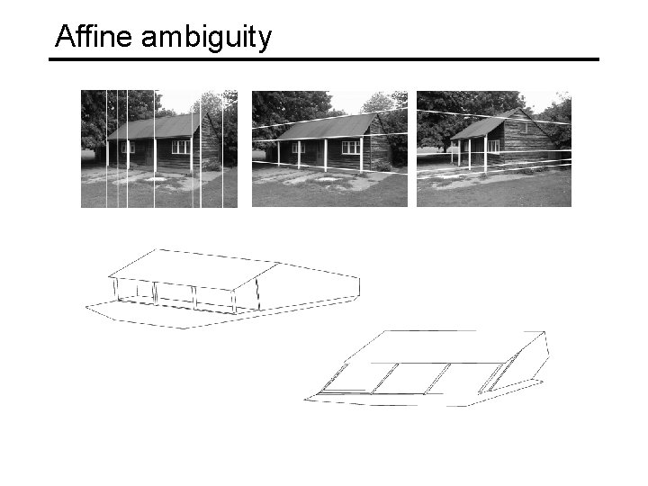
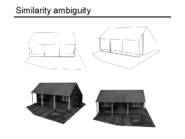
Types of ambiguity Projective 15 dof Preserves intersection and tangency Affine 12 dof Preserves parallellism, volume ratios Similarity 7 dof Preserves angles, ratios of length Euclidean 6 dof Preserves angles, lengths • With no constraints on the camera calibration matrix or on the scene, we get a projective reconstruction • Need additional information to upgrade the reconstruction to affine, similarity, or Euclidean

Projective ambiguity

Projective ambiguity

Affine ambiguity Affine

Affine ambiguity

Similarity ambiguity

Similarity ambiguity

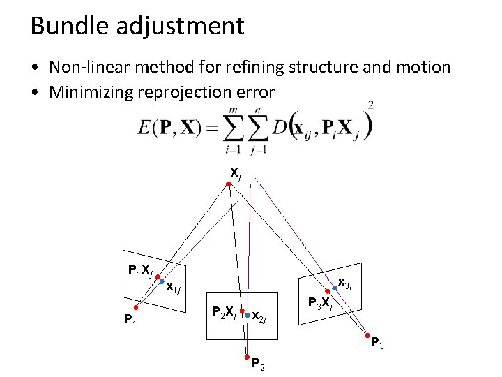
Bundle adjustment • Non-linear method for refining structure and motion • Minimizing reprojection error Xj P 1 x 3 j x 1 j P 2 Xj x 2 j P 3 Xj P 3 P 2

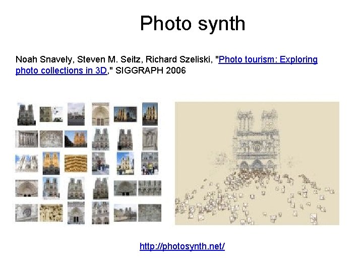
Photo synth Noah Snavely, Steven M. Seitz, Richard Szeliski, "Photo tourism: Exploring photo collections in 3 D, " SIGGRAPH 2006 http: //photosynth. net/

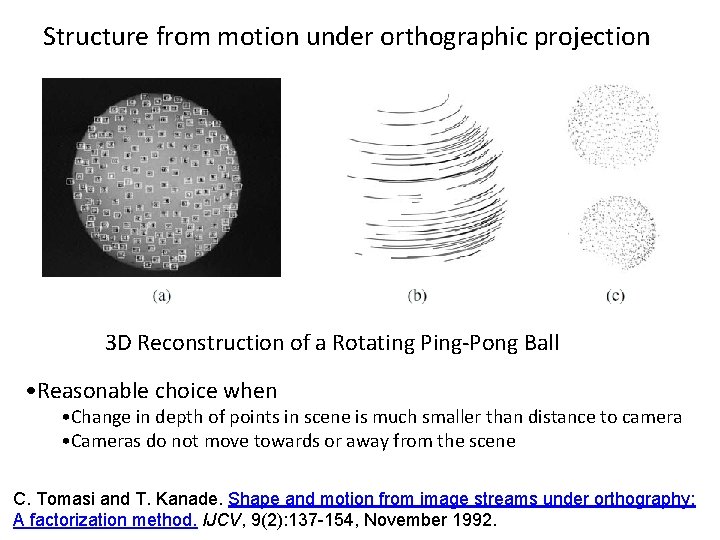
Structure from motion under orthographic projection 3 D Reconstruction of a Rotating Ping-Pong Ball • Reasonable choice when • Change in depth of points in scene is much smaller than distance to camera • Cameras do not move towards or away from the scene C. Tomasi and T. Kanade. Shape and motion from image streams under orthography: A factorization method. IJCV, 9(2): 137 -154, November 1992.

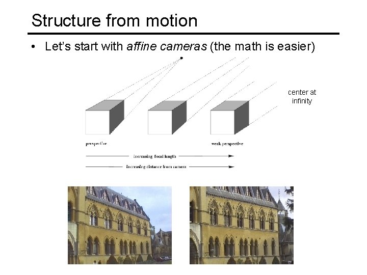
Structure from motion • Let’s start with affine cameras (the math is easier) center at infinity

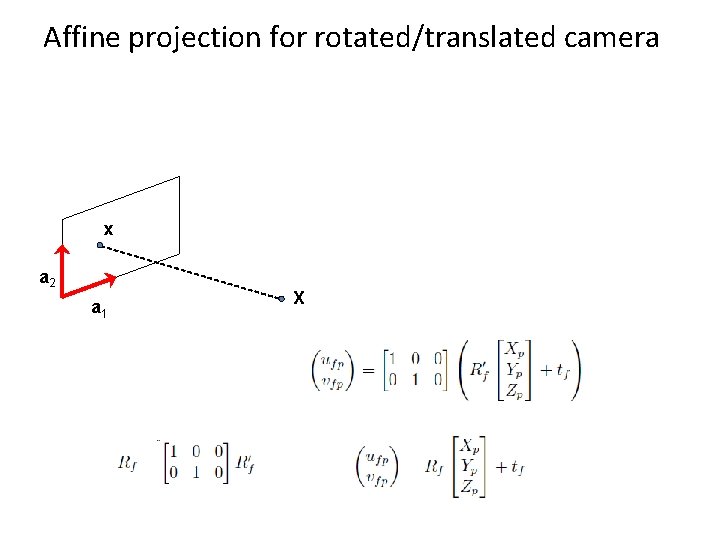
Affine projection for rotated/translated camera x a 2 a 1 X

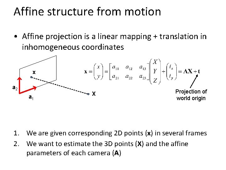
Affine structure from motion • Affine projection is a linear mapping + translation in inhomogeneous coordinates x a 2 a 1 X Projection of world origin 1. We are given corresponding 2 D points (x) in several frames 2. We want to estimate the 3 D points (X) and the affine parameters of each camera (A)

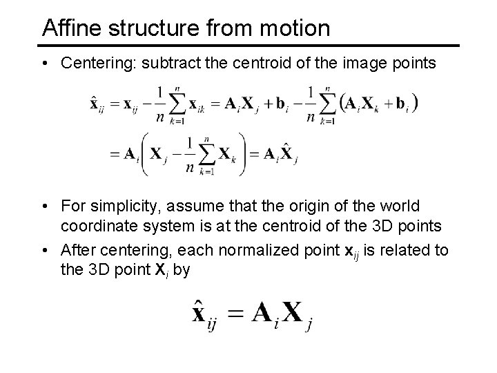
Affine structure from motion • Centering: subtract the centroid of the image points • For simplicity, assume that the origin of the world coordinate system is at the centroid of the 3 D points • After centering, each normalized point xij is related to the 3 D point Xi by

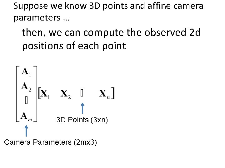
Suppose we know 3 D points and affine camera parameters … then, we can compute the observed 2 d positions of each point 3 D Points (3 xn) Camera Parameters (2 mx 3) 2 D Image Points (2 mxn)

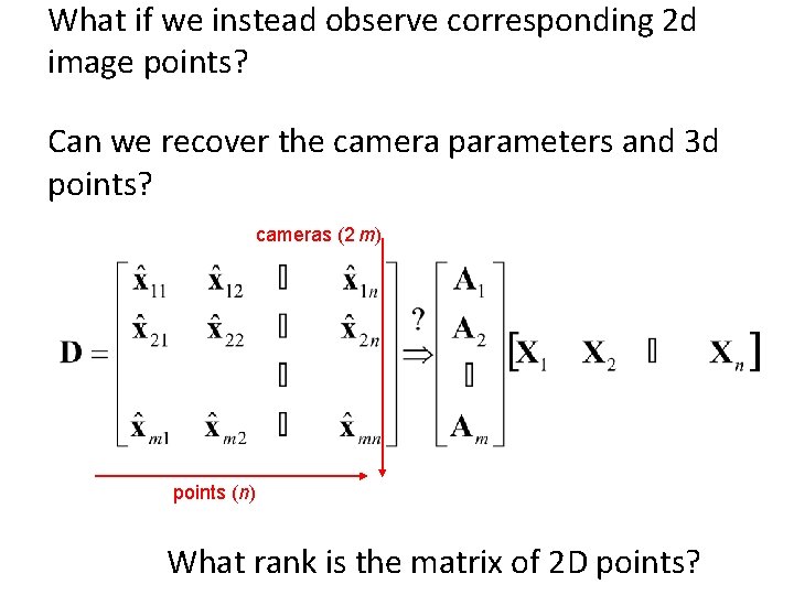
What if we instead observe corresponding 2 d image points? Can we recover the camera parameters and 3 d points? cameras (2 m) points (n) What rank is the matrix of 2 D points?

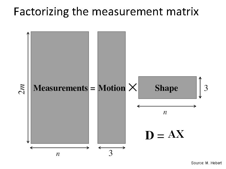
Factorizing the measurement matrix AX Source: M. Hebert

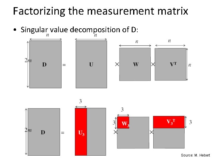
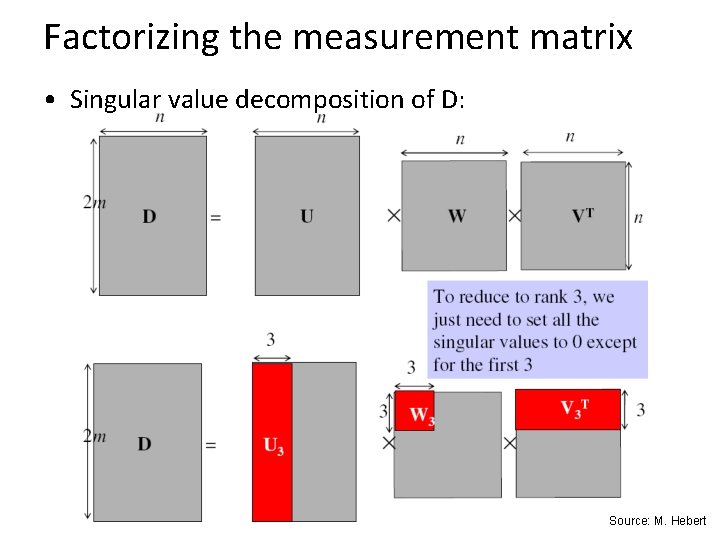
Factorizing the measurement matrix • Singular value decomposition of D: Source: M. Hebert

Factorizing the measurement matrix • Singular value decomposition of D: Source: M. Hebert

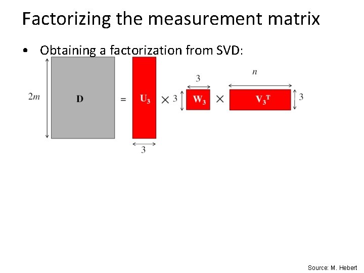
Factorizing the measurement matrix • Obtaining a factorization from SVD: Source: M. Hebert

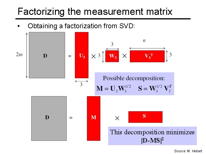
Factorizing the measurement matrix • Obtaining a factorization from SVD: This decomposition minimizes |D-MS|2 Source: M. Hebert

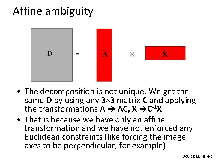
Affine ambiguity • The decomposition is not unique. We get the same D by using any 3× 3 matrix C and applying the transformations A → AC, X →C-1 X • That is because we have only an affine transformation and we have not enforced any Euclidean constraints (like forcing the image axes to be perpendicular, for example) Source: M. Hebert

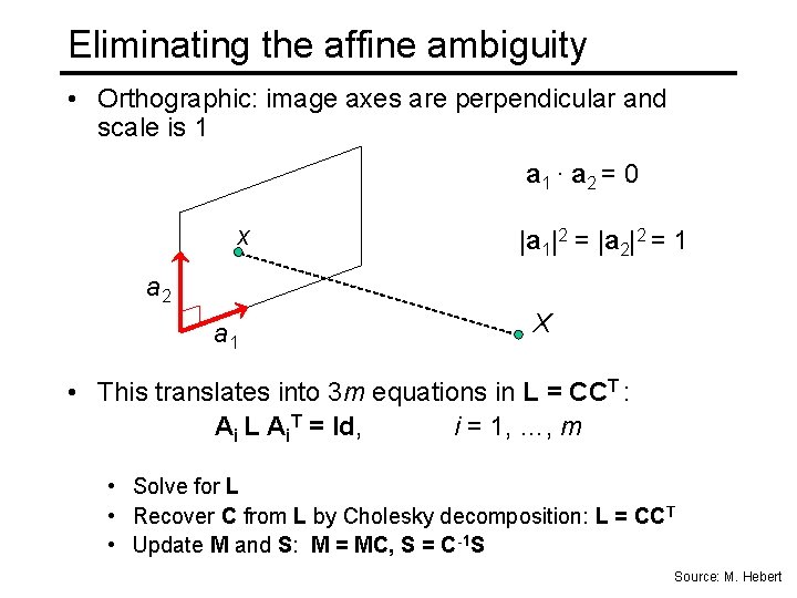
Eliminating the affine ambiguity • Orthographic: image axes are perpendicular and scale is 1 a 1 · a 2 = 0 x |a 1|2 = |a 2|2 = 1 a 2 a 1 X • This translates into 3 m equations in L = CCT : Ai L Ai. T = Id, i = 1, …, m • Solve for L • Recover C from L by Cholesky decomposition: L = CCT • Update M and S: M = MC, S = C-1 S Source: M. Hebert

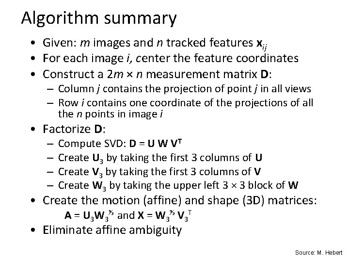
Algorithm summary • Given: m images and n tracked features xij • For each image i, center the feature coordinates • Construct a 2 m × n measurement matrix D: – Column j contains the projection of point j in all views – Row i contains one coordinate of the projections of all the n points in image i • Factorize D: – – Compute SVD: D = U W VT Create U 3 by taking the first 3 columns of U Create V 3 by taking the first 3 columns of V Create W 3 by taking the upper left 3 × 3 block of W • Create the motion (affine) and shape (3 D) matrices: A = U 3 W 3½ and X = W 3½ V 3 T • Eliminate affine ambiguity Source: M. Hebert

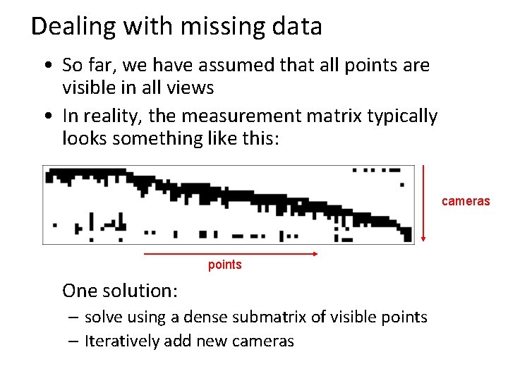
Dealing with missing data • So far, we have assumed that all points are visible in all views • In reality, the measurement matrix typically looks something like this: cameras points One solution: – solve using a dense submatrix of visible points – Iteratively add new cameras

A nice short explanation • Class notes from Lischinksi and Gruber http: //www. cs. huji. ac. il/~csip/sfm. pdf

Reconstruction results (project 5) C. Tomasi and T. Kanade. Shape and motion from image streams under orthography: A factorization method. IJCV, 9(2): 137 -154, November 1992.

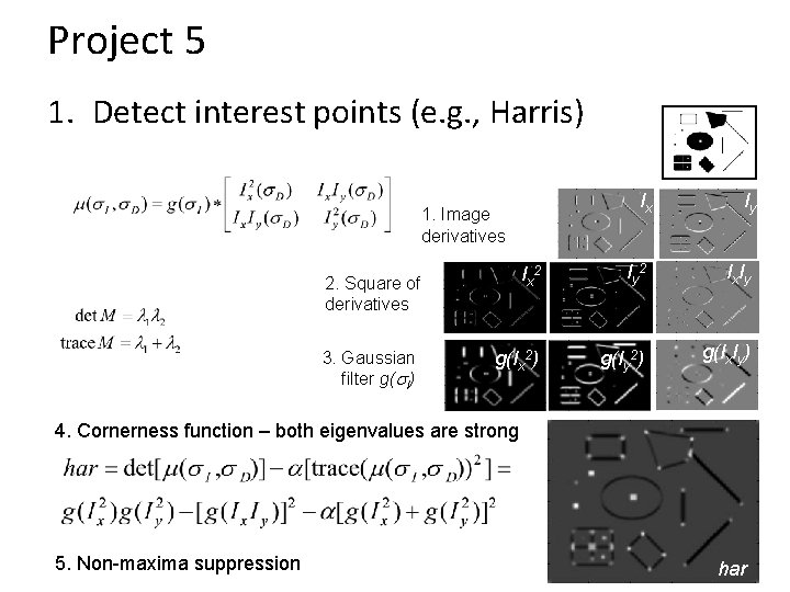
Project 5 1. Detect interest points (e. g. , Harris) Ix Iy Ix 2 Iy 2 Ix Iy g(Ix 2) g(Iy 2) g(Ix. Iy) 1. Image derivatives 2. Square of derivatives 3. Gaussian filter g(s. I) 4. Cornerness function – both eigenvalues are strong 5. Non-maxima suppression 44 har

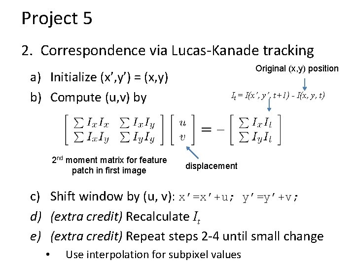
Project 5 2. Correspondence via Lucas-Kanade tracking a) Initialize (x’, y’) = (x, y) b) Compute (u, v) by 2 nd moment matrix for feature patch in first image Original (x, y) position It = I(x’, y’, t+1) - I(x, y, t) displacement c) Shift window by (u, v): x’=x’+u; y’=y’+v; d) (extra credit) Recalculate It e) (extra credit) Repeat steps 2 -4 until small change • Use interpolation for subpixel values

Project 5 3. Get Affine camera matrix and 3 D points using Tomasi-Kanade factorization Solve for orthographic constraints

Project 5 • Tips – Helpful matlab functions: interp 2, meshgrid, ordfilt 2 (for getting local maximum), svd, chol – When selecting interest points, must choose appropriate threshold on Harris criteria or the smaller eigenvalue, or choose top N points – Vectorize to make tracking fast (interp 2 will be the bottleneck) – Get tracking working on one point for a few frames before trying to get it working for all points