11 Conditional Density Functions and Conditional Expected Values

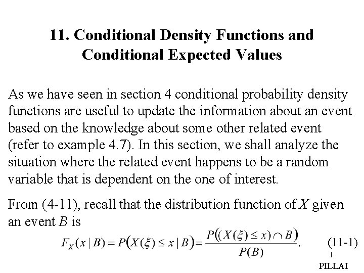
11. Conditional Density Functions and Conditional Expected Values As we have seen in section 4 conditional probability density functions are useful to update the information about an event based on the knowledge about some other related event (refer to example 4. 7). In this section, we shall analyze the situation where the related event happens to be a random variable that is dependent on the one of interest. From (4 -11), recall that the distribution function of X given an event B is (11 -1) 1 PILLAI

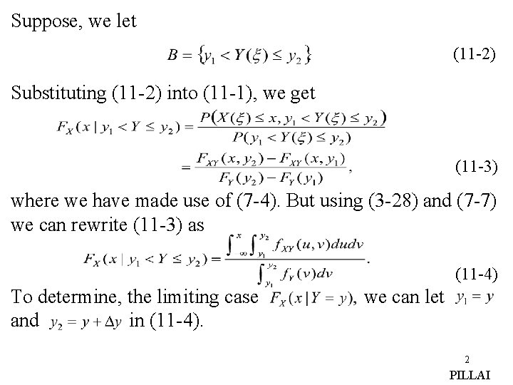
Suppose, we let (11 -2) Substituting (11 -2) into (11 -1), we get (11 -3) where we have made use of (7 -4). But using (3 -28) and (7 -7) we can rewrite (11 -3) as (11 -4) To determine, the limiting case and in (11 -4). we can let 2 PILLAI

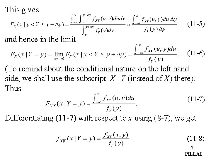
This gives (11 -5) and hence in the limit (11 -6) (To remind about the conditional nature on the left hand side, we shall use the subscript X | Y (instead of X) there). Thus (11 -7) Differentiating (11 -7) with respect to x using (8 -7), we get (11 -8) 3 PILLAI

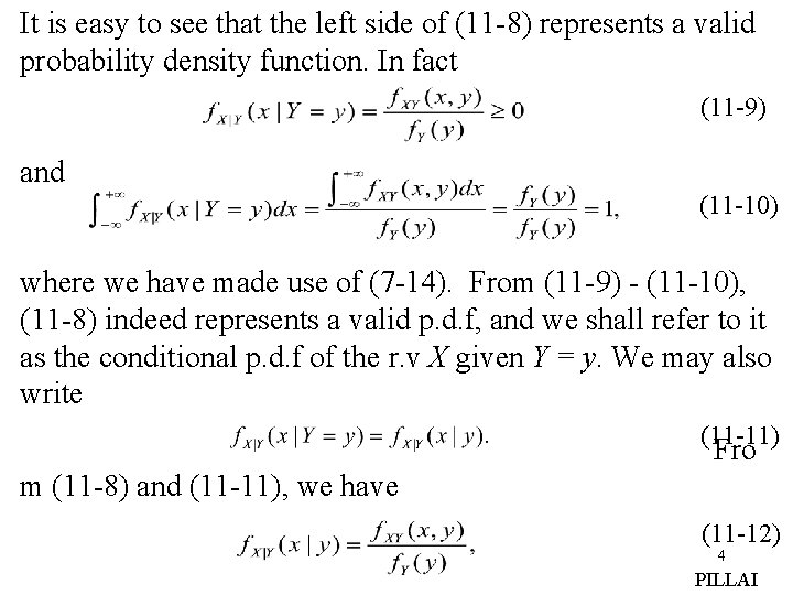
It is easy to see that the left side of (11 -8) represents a valid probability density function. In fact (11 -9) and (11 -10) where we have made use of (7 -14). From (11 -9) - (11 -10), (11 -8) indeed represents a valid p. d. f, and we shall refer to it as the conditional p. d. f of the r. v X given Y = y. We may also write (11 -11) Fro m (11 -8) and (11 -11), we have (11 -12) 4 PILLAI

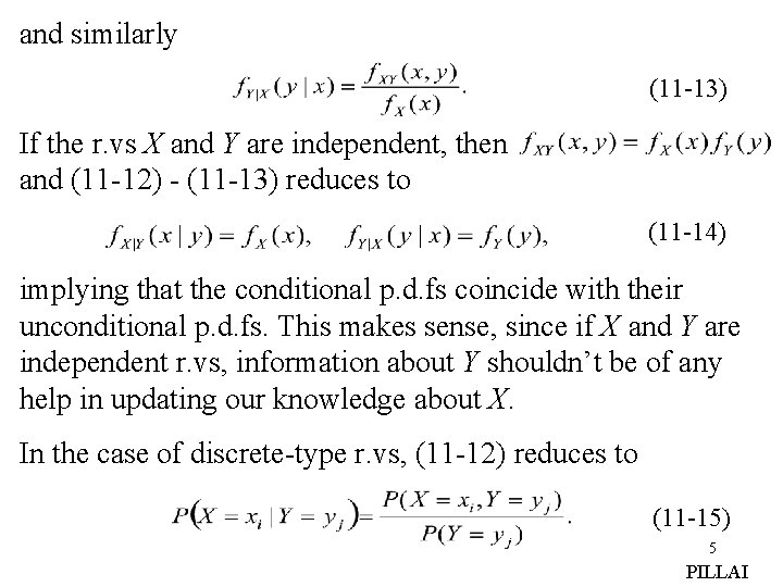
and similarly (11 -13) If the r. vs X and Y are independent, then and (11 -12) - (11 -13) reduces to (11 -14) implying that the conditional p. d. fs coincide with their unconditional p. d. fs. This makes sense, since if X and Y are independent r. vs, information about Y shouldn’t be of any help in updating our knowledge about X. In the case of discrete-type r. vs, (11 -12) reduces to (11 -15) 5 PILLAI

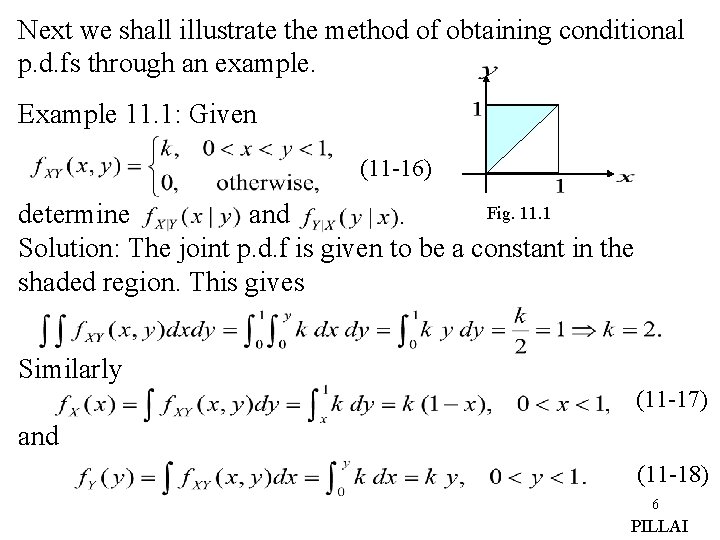
Next we shall illustrate the method of obtaining conditional p. d. fs through an example. Example 11. 1: Given (11 -16) Fig. 11. 1 determine and Solution: The joint p. d. f is given to be a constant in the shaded region. This gives Similarly (11 -17) and (11 -18) 6 PILLAI

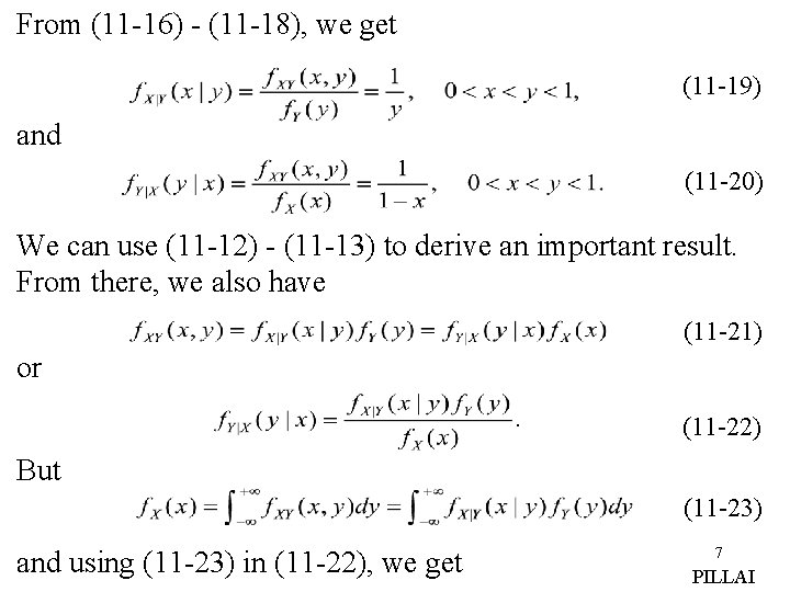
From (11 -16) - (11 -18), we get (11 -19) and (11 -20) We can use (11 -12) - (11 -13) to derive an important result. From there, we also have (11 -21) or (11 -22) But (11 -23) and using (11 -23) in (11 -22), we get 7 PILLAI

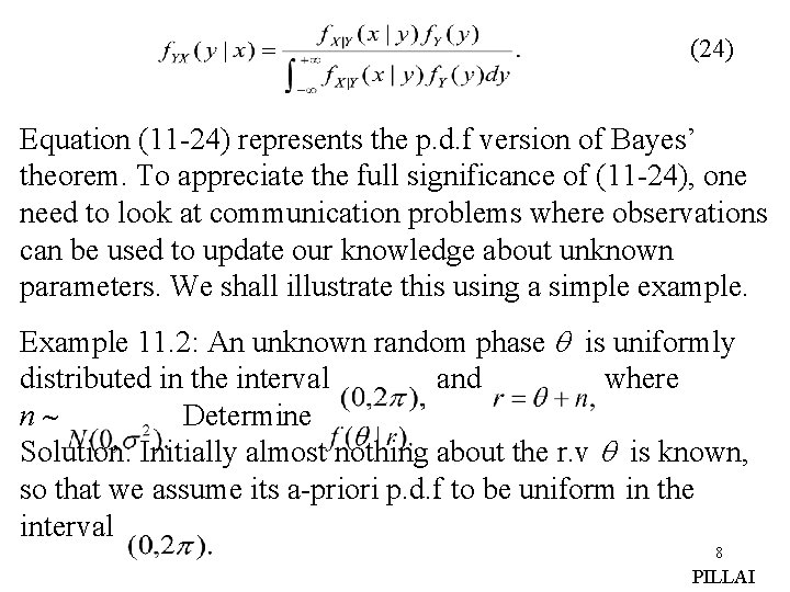
(24) Equation (11 -24) represents the p. d. f version of Bayes’ theorem. To appreciate the full significance of (11 -24), one need to look at communication problems where observations can be used to update our knowledge about unknown parameters. We shall illustrate this using a simple example. Example 11. 2: An unknown random phase is uniformly distributed in the interval and where n Determine Solution: Initially almost nothing about the r. v is known, so that we assume its a-priori p. d. f to be uniform in the interval 8 PILLAI

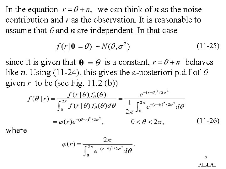
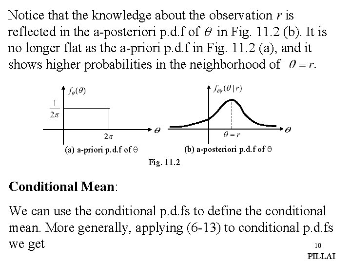
In the equation we can think of n as the noise contribution and r as the observation. It is reasonable to assume that and n are independent. In that case (11 -25) since it is given that is a constant, behaves like n. Using (11 -24), this gives the a-posteriori p. d. f of given r to be (see Fig. 11. 2 (b)) (11 -26) where 9 PILLAI

Notice that the knowledge about the observation r is reflected in the a-posteriori p. d. f of in Fig. 11. 2 (b). It is no longer flat as the a-priori p. d. f in Fig. 11. 2 (a), and it shows higher probabilities in the neighborhood of (b) a-posteriori p. d. f of (a) a-priori p. d. f of Fig. 11. 2 Conditional Mean: We can use the conditional p. d. fs to define the conditional mean. More generally, applying (6 -13) to conditional p. d. fs 10 we get PILLAI

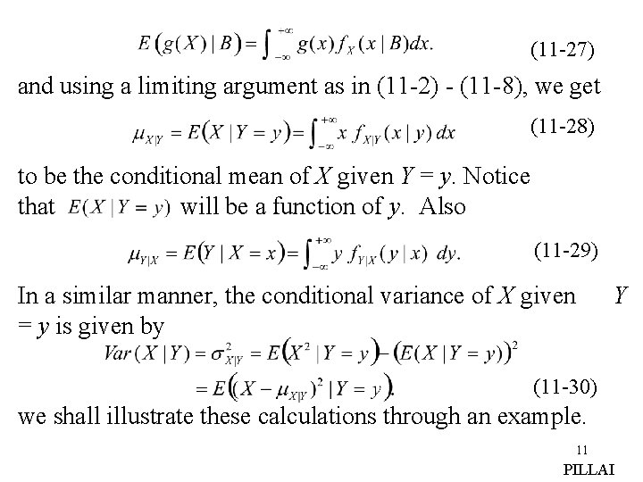
(11 -27) and using a limiting argument as in (11 -2) - (11 -8), we get (11 -28) to be the conditional mean of X given Y = y. Notice that will be a function of y. Also (11 -29) In a similar manner, the conditional variance of X given = y is given by Y (11 -30) we shall illustrate these calculations through an example. 11 PILLAI

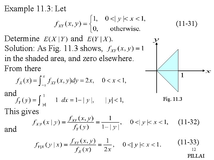
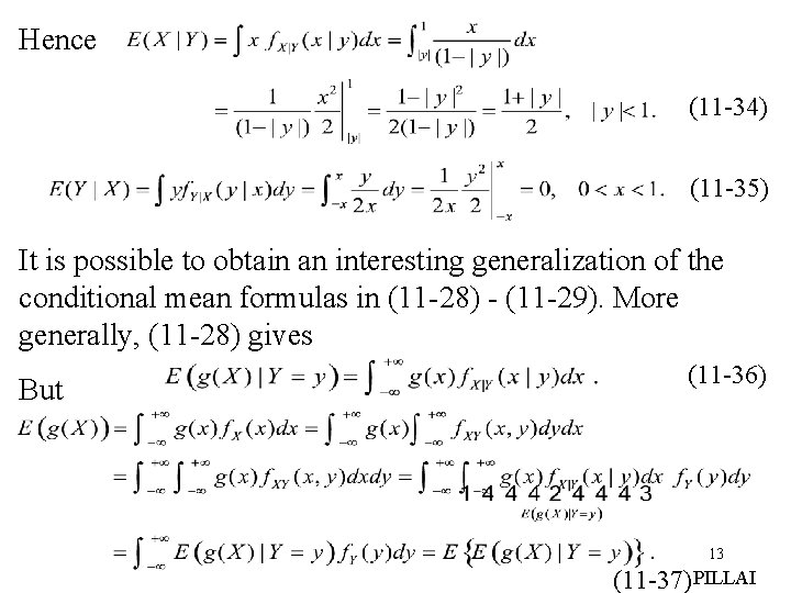
Example 11. 3: Let (11 -31) Determine and Solution: As Fig. 11. 3 shows, in the shaded area, and zero elsewhere. From there and Fig. 11. 3 This gives and (11 -32) (11 -33) 12 PILLAI

Hence (11 -34) (11 -35) It is possible to obtain an interesting generalization of the conditional mean formulas in (11 -28) - (11 -29). More generally, (11 -28) gives But (11 -36) 13 (11 -37) PILLAI

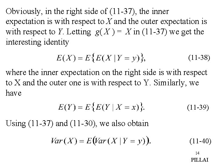
Obviously, in the right side of (11 -37), the inner expectation is with respect to X and the outer expectation is with respect to Y. Letting g( X ) = X in (11 -37) we get the interesting identity (11 -38) where the inner expectation on the right side is with respect to X and the outer one is with respect to Y. Similarly, we have (11 -39) Using (11 -37) and (11 -30), we also obtain (11 -40) 14 PILLAI

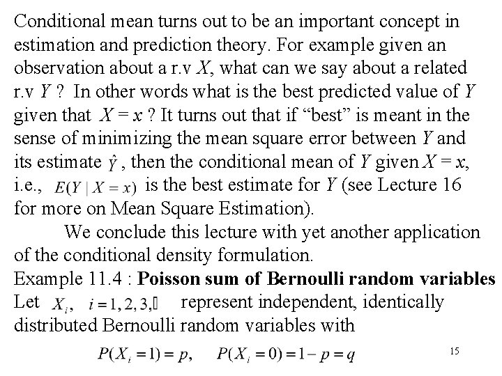
Conditional mean turns out to be an important concept in estimation and prediction theory. For example given an observation about a r. v X, what can we say about a related r. v Y ? In other words what is the best predicted value of Y given that X = x ? It turns out that if “best” is meant in the sense of minimizing the mean square error between Y and its estimate , then the conditional mean of Y given X = x, i. e. , is the best estimate for Y (see Lecture 16 for more on Mean Square Estimation). We conclude this lecture with yet another application of the conditional density formulation. Example 11. 4 : Poisson sum of Bernoulli random variables Let represent independent, identically distributed Bernoulli random variables with 15

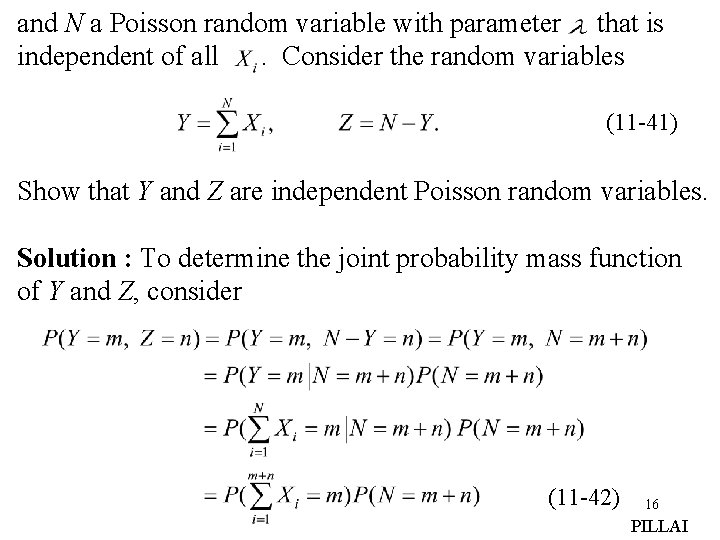
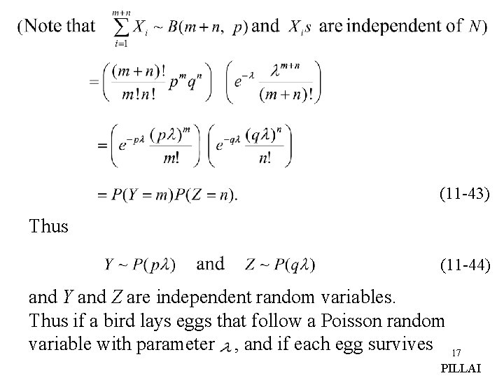
and N a Poisson random variable with parameter that is independent of all. Consider the random variables (11 -41) Show that Y and Z are independent Poisson random variables. Solution : To determine the joint probability mass function of Y and Z, consider (11 -42) 16 PILLAI

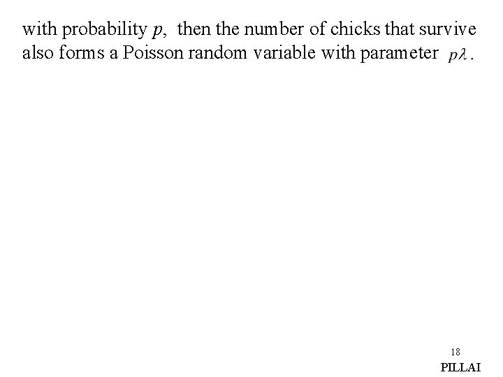
(11 -43) Thus (11 -44) and Y and Z are independent random variables. Thus if a bird lays eggs that follow a Poisson random variable with parameter , and if each egg survives 17 PILLAI

with probability p, then the number of chicks that survive also forms a Poisson random variable with parameter 18 PILLAI