11 A Correlation 11 B Measuring Correlation Unit
11 A Correlation, 11 B Measuring Correlation Unit 3: Statistical Applications 1 11 A, 11 B 2/6/2022 1: 07 PM
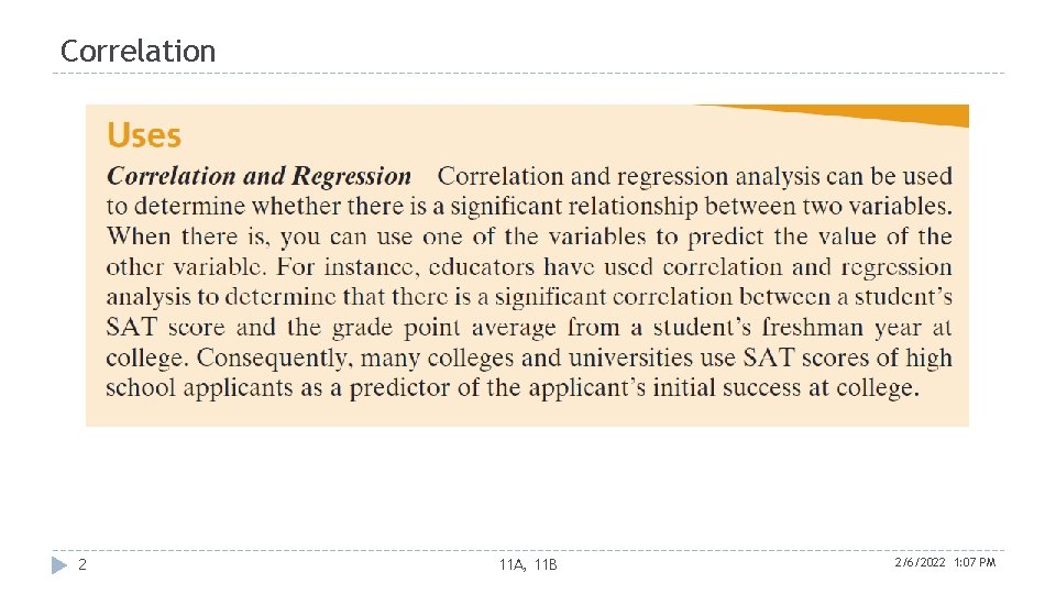
Correlation 2 11 A, 11 B 2/6/2022 1: 07 PM
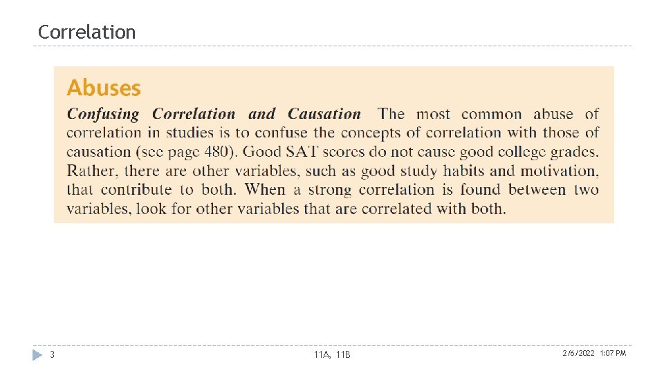
Correlation 3 11 A, 11 B 2/6/2022 1: 07 PM
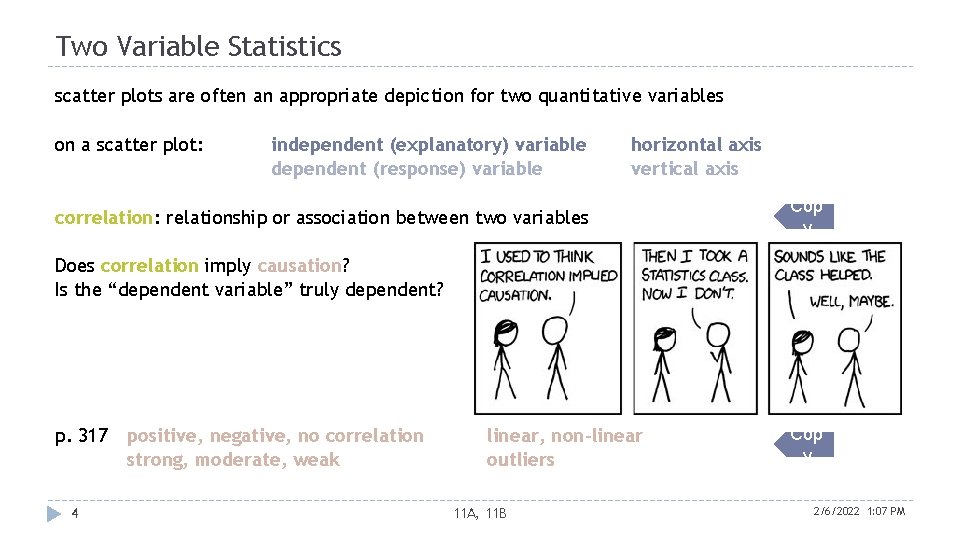
Two Variable Statistics scatter plots are often an appropriate depiction for two quantitative variables on a scatter plot: independent (explanatory) variable dependent (response) variable horizontal axis vertical axis correlation: relationship or association between two variables Cop y Does correlation imply causation? Is the “dependent variable” truly dependent? p. 317 positive, negative, no correlation strong, moderate, weak 4 linear, non-linear outliers 11 A, 11 B Cop y 2/6/2022 1: 07 PM
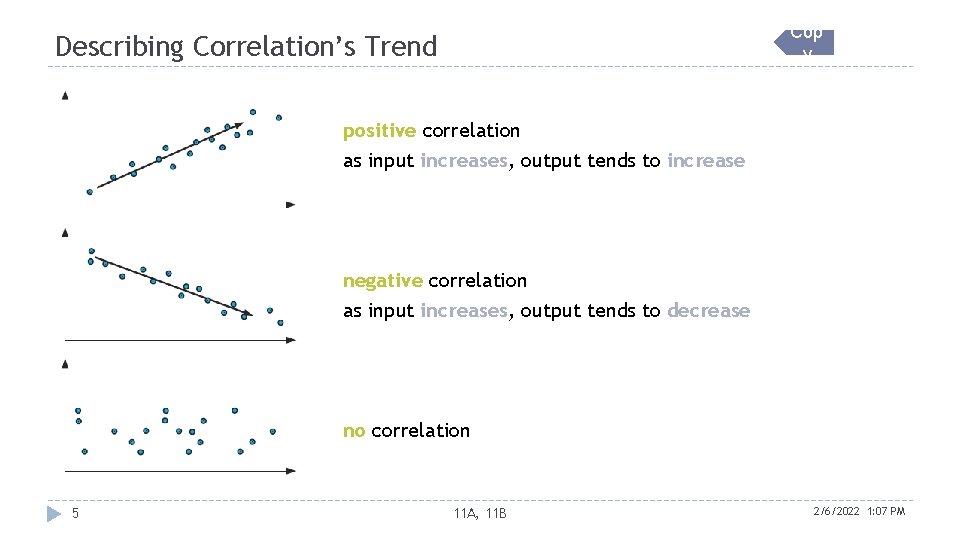
Cop y Describing Correlation’s Trend positive correlation as input increases, output tends to increase negative correlation as input increases, output tends to decrease no correlation 5 11 A, 11 B 2/6/2022 1: 07 PM
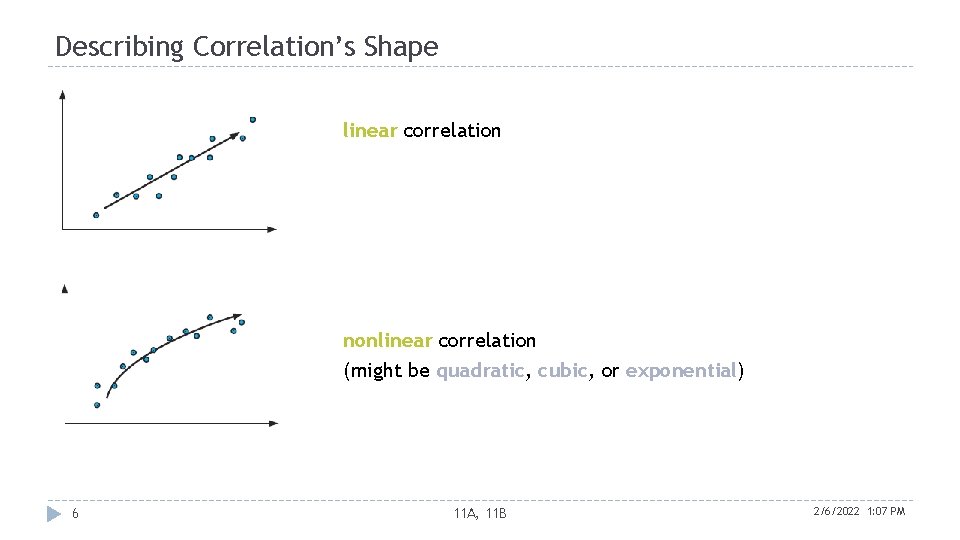
Describing Correlation’s Shape linear correlation nonlinear correlation (might be quadratic, cubic, or exponential) 6 11 A, 11 B 2/6/2022 1: 07 PM
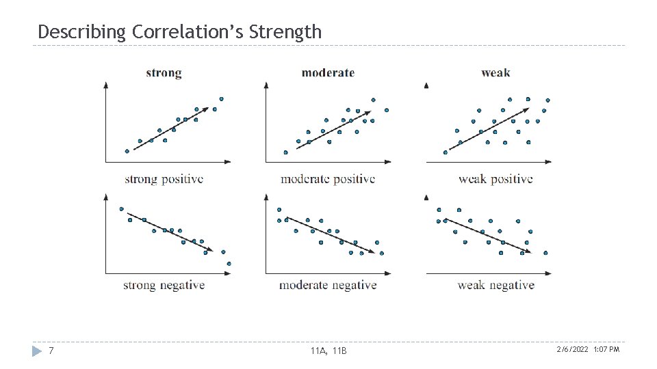
Describing Correlation’s Strength 7 11 A, 11 B 2/6/2022 1: 07 PM
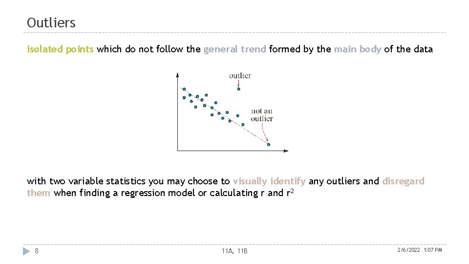
Outliers isolated points which do not follow the general trend formed by the main body of the data with two variable statistics you may choose to visually identify any outliers and disregard them when finding a regression model or calculating r and r 2 8 11 A, 11 B 2/6/2022 1: 07 PM
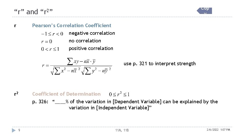
“r” and r Cop y “r 2” Pearson’s Correlation Coefficient negative correlation no correlation positive correlation use p. 321 to interpret strength r 2 Coefficient of Determination p. 326: “____% of the variation in [Dependent Variable] can be explained by the variation in [Independent Variable]” 9 11 A, 11 B 2/6/2022 1: 07 PM
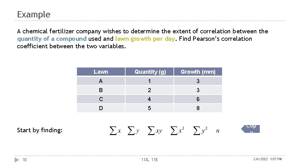
Example A chemical fertilizer company wishes to determine the extent of correlation between the quantity of a compound used and lawn growth per day. Find Pearson’s correlation coefficient between the two variables. Lawn Quantity (g) Growth (mm) A 1 3 B 2 3 C 4 6 D 5 8 Cop y Start by finding: 10 11 A, 11 B 2/6/2022 1: 07 PM
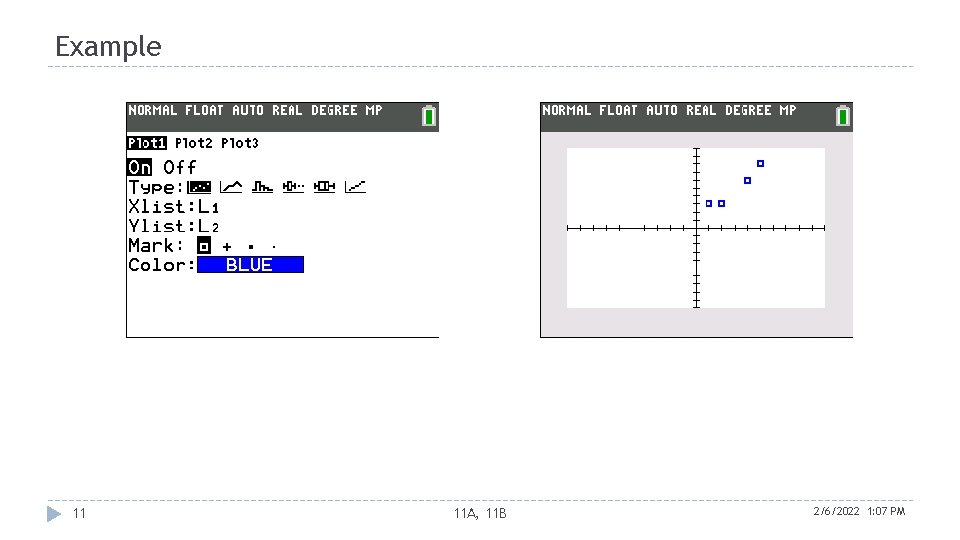
Example 11 11 A, 11 B 2/6/2022 1: 07 PM
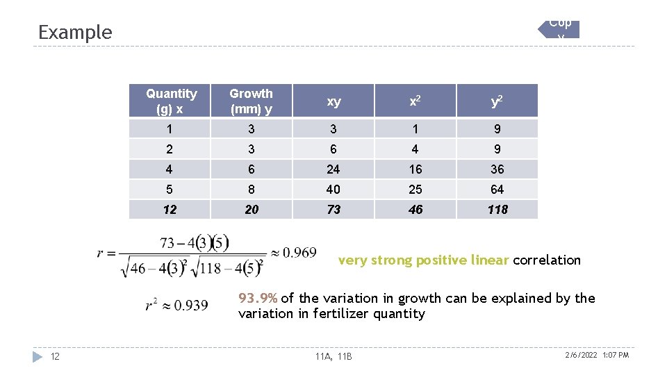
Cop y Example Quantity (g) x Growth (mm) y xy x 2 y 2 1 3 3 1 9 2 3 6 4 9 4 6 24 16 36 5 8 40 25 64 12 20 73 46 118 very strong positive linear correlation 93. 9% of the variation in growth can be explained by the variation in fertilizer quantity 12 11 A, 11 B 2/6/2022 1: 07 PM
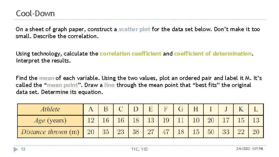
Cool-Down On a sheet of graph paper, construct a scatter plot for the data set below. Don’t make it too small. Describe the correlation. Using technology, calculate the correlation coefficient and coefficient of determination. Interpret the results. Find the mean of each variable. Using the two values, plot an ordered pair and label it M. It’s called the “mean point”. Draw a line through the mean point that “best fits” the original data set. Determine its equation. 13 11 C, 11 D 2/6/2022 1: 07 PM
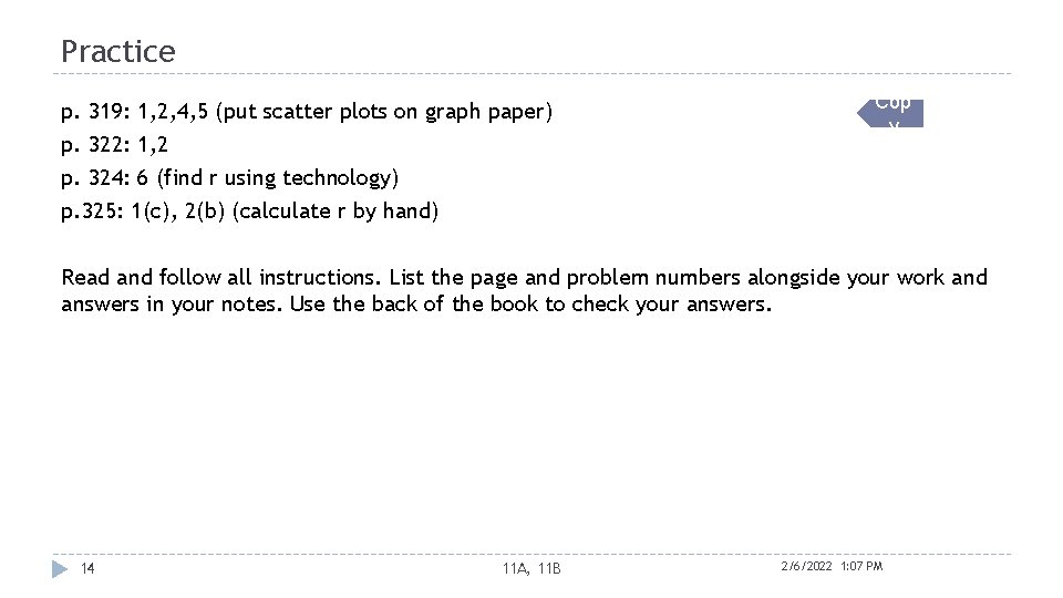
Practice p. 319: 1, 2, 4, 5 (put scatter plots on graph paper) p. 322: 1, 2 Cop y p. 324: 6 (find r using technology) p. 325: 1(c), 2(b) (calculate r by hand) Read and follow all instructions. List the page and problem numbers alongside your work and answers in your notes. Use the back of the book to check your answers. 14 11 A, 11 B 2/6/2022 1: 07 PM
- Slides: 14