11 755 Machine Learning for Signal Processing Latent

Summary So Far n PLCA: q n Sparse Decomposition: q n The notion of

Next up: Shift/Transform Invariance n Sometimes the “typical” structures that compose a sound are

Patches are more representative than frames n n Four bars from a music example

Images: Patches often form the image n A typical image component may be viewed

Shift-invariant modelling n n n A shift-invariant model permits individual bases to be patches

Shift Invariance in one Dimension 5 5 5 98 444 1 2 74453 99

Probability of drawing a particular (t, f) combination n The parameters of the model:

Learning the Model n The parameters of the model are learned analogously to the

Learning the Model n Urn Z and shift T are unknown q q n

Shift invariant model: Update Rules Given data (spectrogram) S(t, f) n n n Initialize

n Shift-invariance in one time: An Example: Two distinct sounds occuring with different repetition

Shift Invariance in Time: Dereverberation + n = Reverberation – a simple model q

Dereverberation n Given the spectrogram of the reverberated signal: q Learn a shift-invariant model

Shift Invariance in Two Dimensions 5 5 5 98 444 1 2 74453 99

Learning the Model n Learning is analogous to the 1 -D case n Given

Learning the Model n Urn Z and shift T, F are unknown q q

2 D Shift Invariance: The problem of indeterminacy n P(t, f|Z) and Ps(T, F|Z)

Example: 2 -D shift invariance n Only one “patch” used to model the image

Example: 2 -D shift invarince The original figure has multiple handwritten renderings of three

Beyond shift-invariance: transform invariance 5 5 5 98 444 1 2 74453 99 15164

Transform invariance: Generation n The set of transforms is enumerable q q E. g.

Transform invariance n The learning algorithm must now estimate q q n n Essentially

Example: Transform Invariance n n Top left: Original figure Bottom left – the two

Transform invariance: model limitations and extensions n The current model only allows one transform

Transform Invariance: Uses and Limitations n Not very useful to analyze audio May be

Example: Higher dimensional n Video example data 11 Oct 2011 11755/18797 32

Slides: 32

Download presentation

11 -755 Machine Learning for Signal Processing Latent Variable Models and Signal Separation Class 12. 11 Oct 2011 11755/18797 1

Summary So Far n PLCA: q n Sparse Decomposition: q n The notion of sparsity and how it can be imposed on learning Sparse Overcomplete Decomposition: q n The basic mixture-multinomial model for audio (and other data) The notion of overcomplete basis set Example-based representations q Using the training data itself as our representation 11 Oct 2011 11755/18797 2

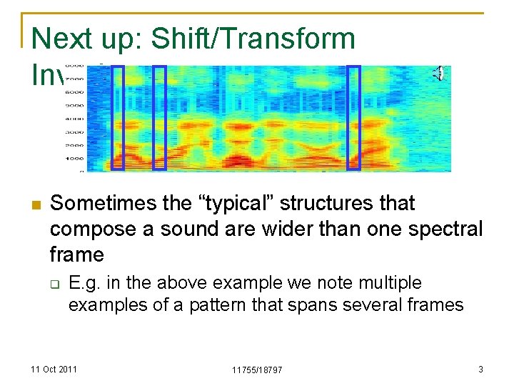
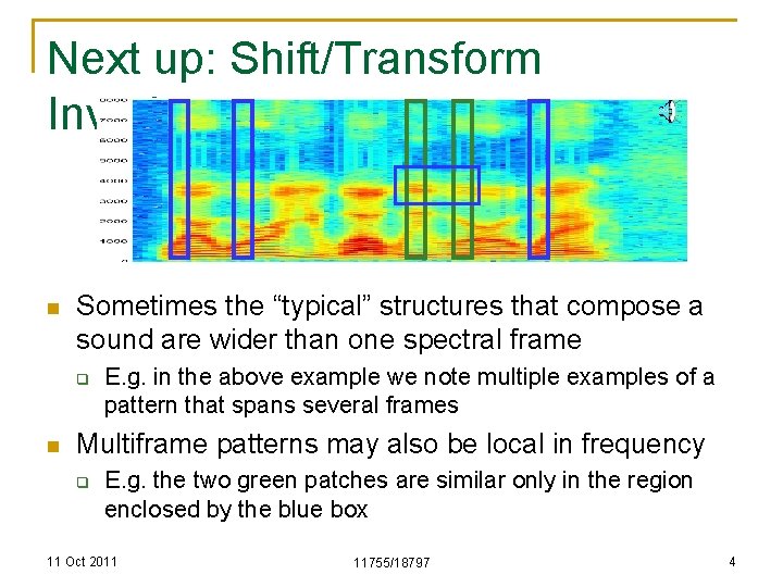
Next up: Shift/Transform Invariance n Sometimes the “typical” structures that compose a sound are wider than one spectral frame q E. g. in the above example we note multiple examples of a pattern that spans several frames 11 Oct 2011 11755/18797 3

Next up: Shift/Transform Invariance n Sometimes the “typical” structures that compose a sound are wider than one spectral frame q n E. g. in the above example we note multiple examples of a pattern that spans several frames Multiframe patterns may also be local in frequency q E. g. the two green patches are similar only in the region enclosed by the blue box 11 Oct 2011 11755/18797 4

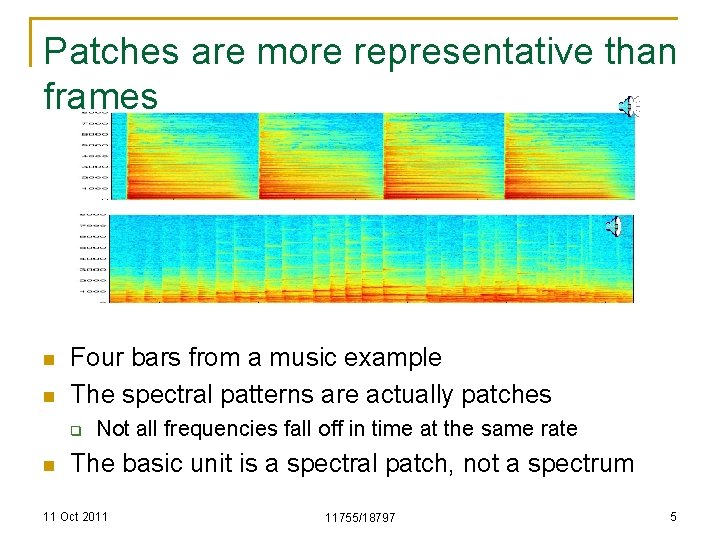
Patches are more representative than frames n n Four bars from a music example The spectral patterns are actually patches q n Not all frequencies fall off in time at the same rate The basic unit is a spectral patch, not a spectrum 11 Oct 2011 11755/18797 5

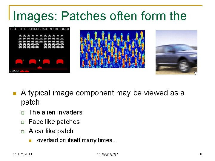
Images: Patches often form the image n A typical image component may be viewed as a patch q q q The alien invaders Face like patches A car like patch n 11 Oct 2011 overlaid on itself many times. . 11755/18797 6

Shift-invariant modelling n n n A shift-invariant model permits individual bases to be patches Each patch composes the entire image. The data is a sum of the compositions from individual patches 11 Oct 2011 11755/18797 7

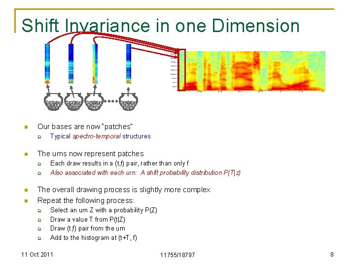
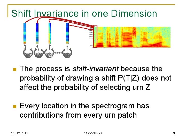
Shift Invariance in one Dimension 5 5 5 98 444 1 2 74453 99 15164 8181 147 3271224 83996 224 47 369 n q n Typical spectro-temporal structures The urns now represent patches q n 91411 502 515 12727 101 203 2469 477 Our bases are now “patches” q n 1 7520 453 37 147381111 2017 37 Each draw results in a (t, f) pair, rather than only f Also associated with each urn: A shift probability distribution P(T|z) The overall drawing process is slightly more complex Repeat the following process: q q Select an urn Z with a probability P(Z) Draw a value T from P(t|Z) Draw (t, f) pair from the urn Add to the histogram at (t+T, f) 11 Oct 2011 11755/18797 8

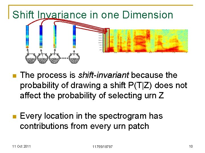
Shift Invariance in one Dimension 5 5 5 98 444 1 2 74453 99 15164 8181 147 3271224 83996 224 47 369 1 7520 453 37 147381111 2017 37 91411 502 515 12727 101 203 2469 477 n The process is shift-invariant because the probability of drawing a shift P(T|Z) does not affect the probability of selecting urn Z n Every location in the spectrogram has contributions from every urn patch 11 Oct 2011 11755/18797 9

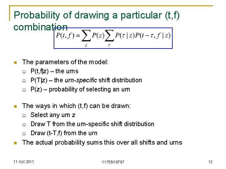
Probability of drawing a particular (t, f) combination n The parameters of the model: q P(t, f|z) – the urns q P(T|z) – the urn-specific shift distribution q P(z) – probability of selecting an urn n The ways in which (t, f) can be drawn: q Select any urn z q Draw T from the urn-specific shift distribution q Draw (t-T, f) from the urn The actual probability sums this over all shifts and urns n 11 Oct 2011 11755/18797 12

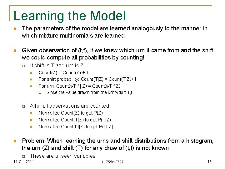
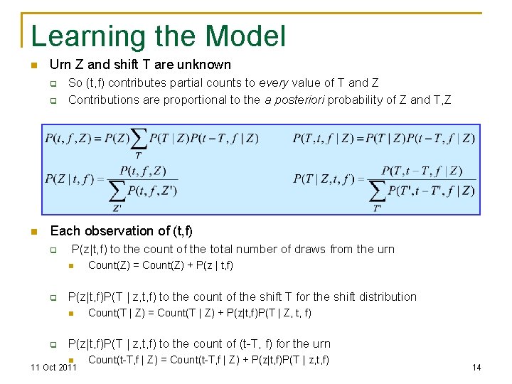
Learning the Model n The parameters of the model are learned analogously to the manner in which mixture multinomials are learned n Given observation of (t, f), it we knew which urn it came from and the shift, we could compute all probabilities by counting! q If shift is T and urn is Z n n n Count(Z) = Count(Z) + 1 For shift probability: Count(T|Z) = Count(T|Z)+1 For urn: Count(t-T, f | Z) = Count(t-T, f|Z) + 1 q q After all observations are counted: n n Since the value drawn from the urn was t-T, f Normalize Count(Z) to get P(Z) Normalize Count(T|Z) to get P(T|Z) Normalize Count(t, f|Z) to get P(t, f|Z) Problem: When learning the urns and shift distributions from a histogram, the urn (Z) and shift (T) for any draw of (t, f) is not known q These are unseen variables 11 Oct 2011 11755/18797 13

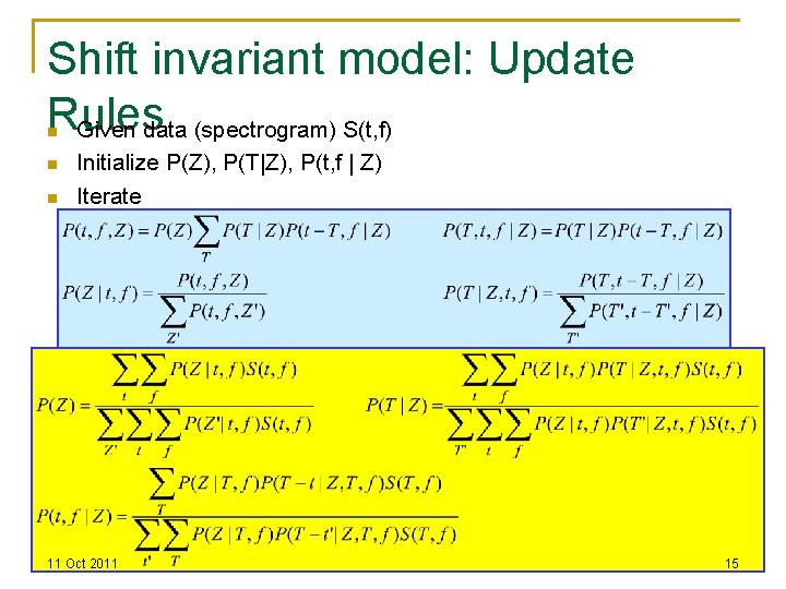
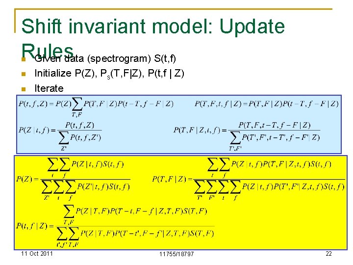
Shift invariant model: Update Rules Given data (spectrogram) S(t, f) n n n Initialize P(Z), P(T|Z), P(t, f | Z) Iterate 11 Oct 2011 11755/18797 15

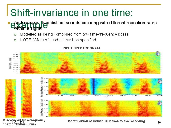
n Shift-invariance in one time: An Example: Two distinct sounds occuring with different repetition rates example within a signal q q Modelled as being composed from two time-frequency bases NOTE: Width of patches must be specified INPUT SPECTROGRAM Discovered time-frequency 11 Oct 2011 “patch” bases (urns) Contribution of individual bases to the recording 11755/18797 16

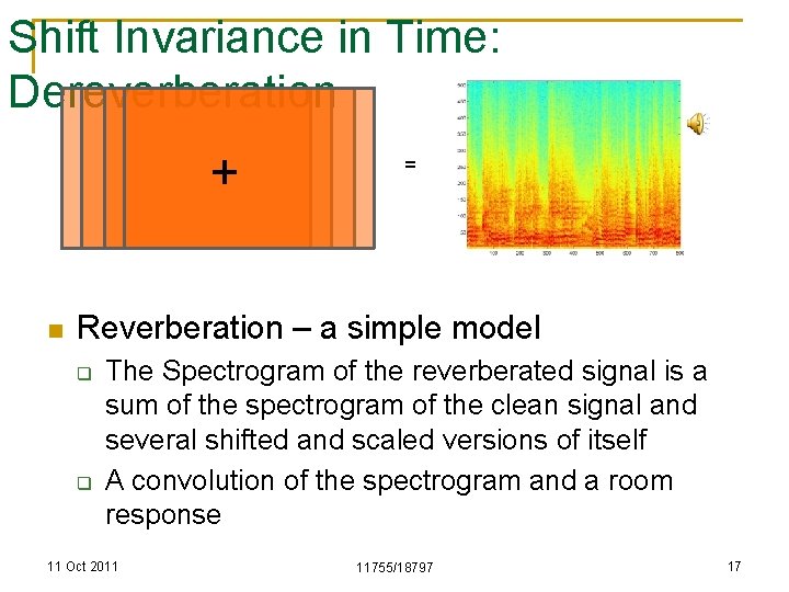
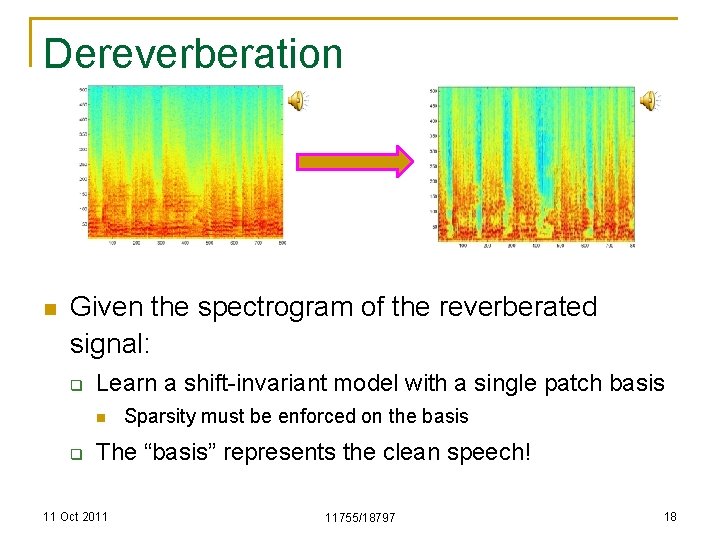
Shift Invariance in Time: Dereverberation + n = Reverberation – a simple model q q The Spectrogram of the reverberated signal is a sum of the spectrogram of the clean signal and several shifted and scaled versions of itself A convolution of the spectrogram and a room response 11 Oct 2011 11755/18797 17

Dereverberation n Given the spectrogram of the reverberated signal: q Learn a shift-invariant model with a single patch basis n q Sparsity must be enforced on the basis The “basis” represents the clean speech! 11 Oct 2011 11755/18797 18

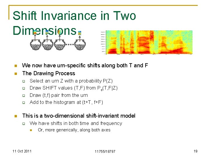
Shift Invariance in Two Dimensions 5 5 5 98 444 1 2 74453 99 15164 8181 147 3271224 83996 224 47 369 n n 91411 502 515 12727 101 203 2469 477 We now have urn-specific shifts along both T and F The Drawing Process q q n 1 7520 453 37 147381111 2017 37 Select an urn Z with a probability P(Z) Draw SHIFT values (T, F) from Ps(T, F|Z) Draw (t, f) pair from the urn Add to the histogram at (t+T, f+F) This is a two-dimensional shift-invariant model q We have shifts in both time and frequency n 11 Oct 2011 Or, more generically, along both axes 11755/18797 19

Learning the Model n Learning is analogous to the 1 -D case n Given observation of (t, f), it we knew which urn it came from and the shift, we could compute all probabilities by counting! q If shift is T, F and urn is Z n n n Count(Z) = Count(Z) + 1 For shift probability: Shift. Count(T, F|Z) = Shift. Count(T, F|Z)+1 For urn: Count(t-T, f-F | Z) = Count(t-T, f-F|Z) + 1 q q After all observations are counted: n n Since the value drawn from the urn was t-T, f-F Normalize Count(Z) to get P(Z) Normalize Shift. Count(T, F|Z) to get Ps(T, F|Z) Normalize Count(t, f|Z) to get P(t, f|Z) Problem: Shift and Urn are unknown 11 Oct 2011 11755/18797 20

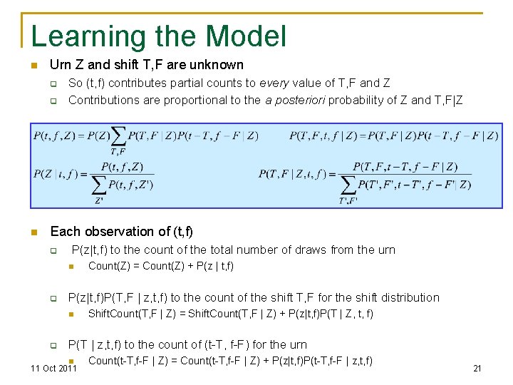
Learning the Model n Urn Z and shift T, F are unknown q q n So (t, f) contributes partial counts to every value of T, F and Z Contributions are proportional to the a posteriori probability of Z and T, F|Z Each observation of (t, f) q P(z|t, f) to the count of the total number of draws from the urn n q P(z|t, f)P(T, F | z, t, f) to the count of the shift T, F for the shift distribution n q Count(Z) = Count(Z) + P(z | t, f) Shift. Count(T, F | Z) = Shift. Count(T, F | Z) + P(z|t, f)P(T | Z, t, f) P(T | z, t, f) to the count of (t-T, f-F) for the urn n 11 Oct 2011 Count(t-T, f-F | Z) = Count(t-T, f-F | Z) + P(z|t, f)P(t-T, f-F | z, t, f) 11755/18797 21

Shift invariant model: Update Rules Given data (spectrogram) S(t, f) n n n Initialize P(Z), Ps(T, F|Z), P(t, f | Z) Iterate 11 Oct 2011 11755/18797 22

2 D Shift Invariance: The problem of indeterminacy n P(t, f|Z) and Ps(T, F|Z) are analogous q n n Difficult to specify which will be the “urn” and which the “shift” Additional constraints required to ensure that one of them is clearly the shift and the other the urn Typical solution: Enforce sparsity on Ps(T, F|Z) q The patch represented by the urn occurs only in a few locations in the data 11 Oct 2011 11755/18797 23

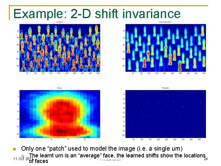
Example: 2 -D shift invariance n Only one “patch” used to model the image (i. e. a single urn) q The learnt urn is an “average” face, the learned shifts show the locations 24 11755/18797 of faces 11 Oct 2011

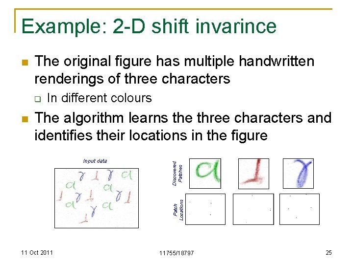
Example: 2 -D shift invarince The original figure has multiple handwritten renderings of three characters q n In different colours The algorithm learns the three characters and identifies their locations in the figure Patch Locations Input data Discovered Patches n 11 Oct 2011 11755/18797 25

Beyond shift-invariance: transform invariance 5 5 5 98 444 1 2 74453 99 15164 8181 147 3271224 83996 224 47 369 n n 1 7520 453 37 147381111 2017 37 91411 502 515 12727 101 203 2469 477 The draws from the urns may not only be shifted, but also transformed The arithmetic remains very similar to the shiftinvariant model q q We must now impose one of an enumerated set of transforms to (t, f), after shifting them by (T, F) In the estimation, the precise transform applied is an unseen variable 11 Oct 2011 11755/18797 26

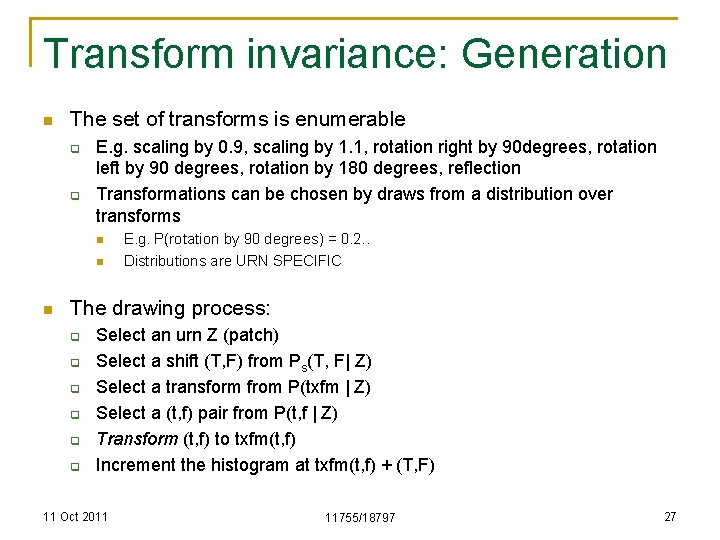
Transform invariance: Generation n The set of transforms is enumerable q q E. g. scaling by 0. 9, scaling by 1. 1, rotation right by 90 degrees, rotation left by 90 degrees, rotation by 180 degrees, reflection Transformations can be chosen by draws from a distribution over transforms n n n E. g. P(rotation by 90 degrees) = 0. 2. . Distributions are URN SPECIFIC The drawing process: q q q Select an urn Z (patch) Select a shift (T, F) from Ps(T, F| Z) Select a transform from P(txfm | Z) Select a (t, f) pair from P(t, f | Z) Transform (t, f) to txfm(t, f) Increment the histogram at txfm(t, f) + (T, F) 11 Oct 2011 11755/18797 27

Transform invariance n The learning algorithm must now estimate q q n n Essentially determines what the basic shapes are, where they occur in the data and how they are transformed The mathematics for learning are similar to the maths for shift invariance q n P(Z) – probability of selecting urn/patch in any draw P(t, f|Z) – the urns / patches P(txfm | Z) – the urn specific distribution over transforms Ps(T, F|Z) – the urn-specific shift distribution With the addition that each instance of a draw must be fractured into urns, shifts AND transforms Details of learning are left as an exercise q Alternately, refer to Madhusudana Shashanka’s Ph. D thesis at BU 11 Oct 2011 11755/18797 28

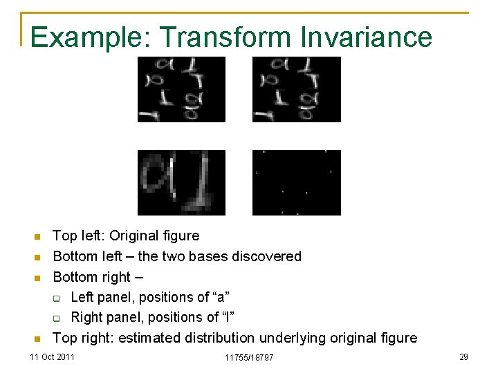
Example: Transform Invariance n n Top left: Original figure Bottom left – the two bases discovered Bottom right – q Left panel, positions of “a” q Right panel, positions of “l” Top right: estimated distribution underlying original figure 11 Oct 2011 11755/18797 29

Transform invariance: model limitations and extensions n The current model only allows one transform to be applied at any draw q n An obvious extension is to permit combinations of transformations q n n E. g. a basis may be rotated or scaled, but not scaled and rotated Model must be extended to draw the combination from some distribution Data dimensionality: All examples so far assume only two dimensions (e. g. in spectrogram or image) The models are trivially extended to higherdimensional data 11 Oct 2011 11755/18797 30

Transform Invariance: Uses and Limitations n Not very useful to analyze audio May be used to analyze images and video n Main restriction: Computational complexity n q q Requires unreasonable amounts of memory and CPU Efficient implementation an open issue 11 Oct 2011 11755/18797 31

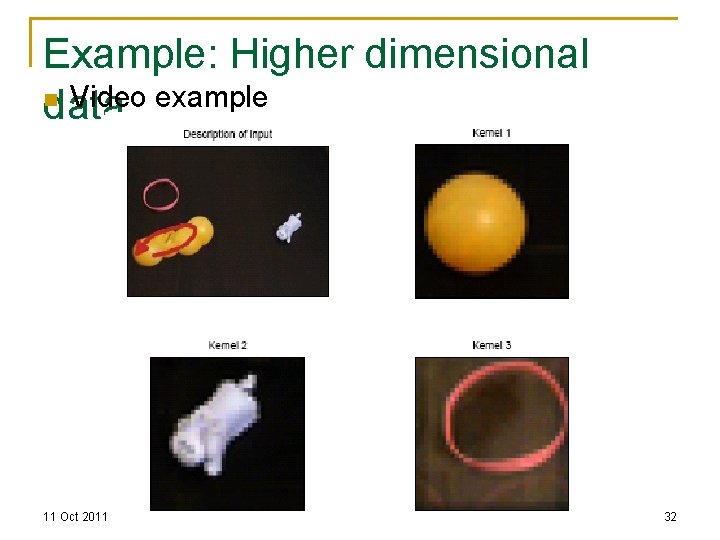
Example: Higher dimensional n Video example data 11 Oct 2011 11755/18797 32